
5.2 Intermediate Table Skills
Learning Objectives
- Filter table data.
- Add a total row to a table.
- Insert subtotals into a table.
FILTERING DATA
When you first create an Excel table, filter arrows appear in all the column headings. We have seen that you can use those arrows to sort your data by a single column. You can also use these same arrows to filter or limit the data you see by narrowing the displayed data within a column. There are many ways to filter data within a column depending on whether the data in the column is text or numeric. Table 5.5 gives you some filter examples:
Table 5.5 Filter Examples
| Text Filters | |||
| Desired Results | Filter Column | Text Filter | Checkbox Selected |
| Data for the State of New Jersey (NJ) | State | Equals NJ | NJ |
| Data for Books that Have Gardening in Their Title | Title | Contains Gardening | |
| Data for Weather on the Weekend | Day | Equals Saturday OR equals Sunday | Saturday and Sunday |
| Numeric Filters | |||
| Desired Results | Filter Column | Number Filter | Checkbox Selected |
| Data for Income Greater Than $1,000 | Income | Greater than 1,000 | |
| Data for Amount Paid Equal to Zero | Amount Paid | Equals 0.00 | 0.00 |
| Data for Mortgage and Auto Loans | Loan Type | Equals Mortgage OR equals Auto | Mortgage and Auto |
Notice there are sometimes more than one way to filter data (i.e. – with a filter choice or a checked box). There are also single criteria filters, as well as, multi-criteria filters. We will explore all of these next.
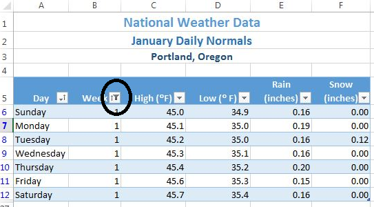
To start filtering, let’s look at just the first week of data in the Weekly OR sheet:
- Click on the Weekly OR sheet and click on a cell in the table.
- Click the filter arrow to the right of the Week heading.
- Click the Select All checkbox to deselect all of the checkbox choices.
- Click on 1 to select Week 1.
- Click OK.
Your table should look like Figure 5.16. You should see only 7 rows of Week 1 data in your table. Notice in your Status Bar at the bottom of your screen the message “7 of 31 records found”. Also notice that the filter arrow in the Week heading has changed to a funnel which indicates that this column is currently filtered.
- Click the funnel next to the Week heading.
- Select “Clear filter from Week”.
Skill Refresher
Filter a Column
- Click the filter arrow to the right of the heading in the column you want to filter.
- Click the Select All checkbox to deselect all of the checkbox choices.
- Click on the checkboxes you want to filter by.
- Click OK.
Un-Filter a Column
- Click the funnel to the right of the heading in the column you filtered.
- Select Clear filter.
- Click in the Portland ME sheet, then click on a cell in the table.
- Click on the filter arrow next to the High heading.
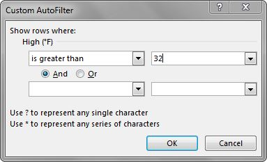
- Click on Number filters, then select Greater than. The Custom AutoFilter dialog box will appear on your screen.
- Enter 32 in the space to the right of “is Greater than”. Your Custom AutoFilter dialog box should now match Figure 5.17.

Figure 5.17 AutoFilter Dialog Box - Click OK.
You should see that it was only above 32 degrees three days in January in Maine – the first three! Check your table against Figure 5.18.
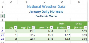
Figure 5.18 Filter Results
Let’s review sorting and filtering in the following steps:
- Click on the Weekly OR sheet and clear the Day column filter.
- Sort the table by Week (smallest to largest).
- Filter the table to only show Mondays.
- Compare your table results to Figure 5.19.
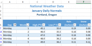
Figure 5.19 Filter Results

Filtering using the Slicer
Beginning in Excel 2013, slicers were added to the software as another way to filter your table data. A slicer is really useful because it clearly indicates what data is shown in your table after you filter your data.
Let’s try using the Slicer to filter our Portland OR data table:
- Click on the Portland OR sheet and click in the table.
- In the ribbon’s Table Tools Design tab, click Insert Slicer.
- Click on Day in the Insert Slicers dialog box, and then click OK.
- Drag the slicer so that the upper left-hand corner lines up with the top corner of cell G5.
- Notice that when you insert a Slicer, a Slicer Options tab appears on the ribbon. This tab lets you change the style and size of the entire slicer or the individual slicer buttons.
- Click on the Slicer options tab, then click on the More button next to Slicer Styles. The choices in Figure 5.20 will show on your screen.
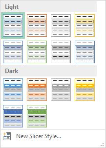
- Select the first choice under Dark.
- In the Size group on the Slicer Options ribbon (NOT the Buttons group), change the width to 1”.
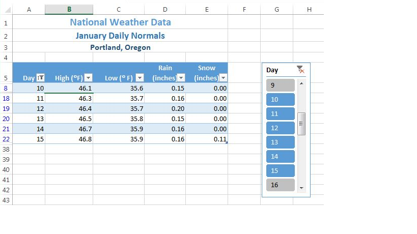
- Click in the table and scroll down to Day 15 and click the 15 button to show only the data for January 15th in the table.
- Hold down the CTRL key and click on the Slicer buttons for Days 10 through 14. Your table should now show the data from Days 10-15.
- Sort the Day column in Ascending order to show the days in order as in Figure 5.21.
Total Rows
By adding a total row to the bottom of your table, you can quickly see summary data for one or more of the columns in your table. Total rows can be added to tables as a whole, or those that are filtered. Total rows can easily be toggled on and off as the need for summary data arises.
- Click on the Portland ME sheet and clear the filter from the High column.
- Click on the Total Row check box in the Table Style Options group in the Table Tools Design tab in the ribbon.
- Scroll to the bottom of your table to the Total Row. Notice the total for the Snow data.
- Click on D37 (in the Rain column), and then click the down-arrow that appears to the right of the cell.
- Choose Sum to add a sum to the Total Row in the Rain column.
- To see the Average rainfall for the month of January, click on the arrow again and choose Average.
- Repeat this step in E37 to see the Average snowfall.
- Use the Decrease Decimal button in the Home tab of the ribbon to change the decimal places in D37 and E37 to 2. Compare your Total Row to Figure 5.22.

- Now switch to the Weekly OR sheet and see if you can successfully add a Slicer and Total Row to this table:
- Clear the filter from the Day column.
- Add a Slicer for the Day column to the sheet.
- Move the top left corner of the slicer to H5. Resize it as needed and choose a Slicer Style.
- Select Monday through Friday in the Slicer so that Saturday and Sunday data do NOT show in your table.
- Add a Total Row that averages the High and Low columns. Your averages should be High: 47.0 and Low: 35.8. Change the label “Total” to “Average” by clicking A37 and typing Average.
Skill Refresher
Add a Total Row
- Click on the Total Row check box in the Table Style Options group in the Table Tools Design tab in the ribbon.
- Scroll to the bottom of your table to find the Total Row.
- Click in one of the columns in the Total Row, and then click the down-arrow that appears to the right of the cell.
- Choose Sum to add a sum to the Total Row in the column.
- To see the Average for column, click on the arrow again and choose Average.
Some other choices in the Total Row are Count (for words), Count Numbers, Max, and Min.
Skill Refresher
Add a Slicer
- Click on Insert Slicer in the Table Tools Design tab in the ribbon.
- Check the box for the column to which you want to add a Slicer.
- Click OK.
Subtotaling
You can automatically calculate subtotals and grand totals in a table for a column. This is a powerful tool that allows you to quickly display multiple levels of summary data within your table. This can provide Management with a report of higher level summary data one minute, and then can be easily switched back to detailed data the next minute. It is important to save often during this process and follow the steps carefully. It is recommended that you make a copy of the data you want to subtotal and place it in a new sheet, so that you can save the summary subtotaled data separately if desired.
In order to subtotal successfully, you always need to do the following in order:
- Sort by the column you want to subtotal on.
- Convert the table back to a normal Excel range. You cannot subtotal inside a table.
- Subtotal in the Data tab in the ribbon.
- If you want to limit your displayed data further, Filter in the Data tab in the ribbon.
We want to find out what the weather looks like for each day of the week, so we’ll need to save our data to a new sheet, sort by the days of the week, and then convert the table in order to get ready to see the subtotal.
- Click on the Weekly OR sheet.
- Point at the Weekly OR sheet tab at the bottom of the screen, hold the CTRL key down, and left-drag the sheet to the right until you are past all the existing sheets.
- When you see a sheet icon with a + sign, let go of the mouse button and then the CTRL key. A Weekly OR (2) sheet will appear.
- Right-click on the new Sheet tab, select Rename, type Subtotal OR, and then press ENTER.
- Save your file before you start Subtotaling!
- Remove all filters in the table by clicking the Data tab and then choosing Clear.
- Now we want to Sort the table by the Day column using a Custom Sort in the Sort button in the ribbon to sort in the order Sunday, Monday, Tuesday, etc. (See Figure 5.13 through 5.15 for a review of Custom Sorting.)
- Before you can subtotal, you must convert your table back to a regular range. To do this, click Convert to Range in the Table Tools Design tab on the ribbon. (See Figure 5.23)
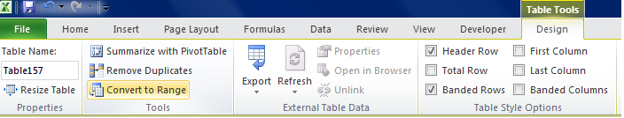
Figure 5.23 Convert to Range
- When asked if you want to convert the table, click Yes.
- Because your data is no longer formatted as a table, your slicer will disappear; and you will no longer have access to the Table Tools Design tab in the ribbon.
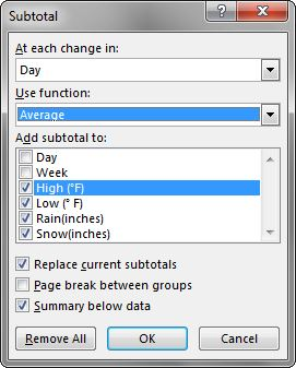
- Under the Data tab in the ribbon, click Subtotal.
- In the Subtotal Window, make the choices shown in the Figure 5.24. It is essential that you select the column you sorted by in the “At each change in” field at the top of the window. Click OK.
Your data should look like Figure 5.25. Successful subtotaling shows only one subtotal for each group in the column you sorted by. (HINT: If you end up with more than one Subtotal for the same group (i.e – one of the days of the week in our example), you did not sort before subtotaling. Remove your subtotals using the Remove All button in Figure 5.24, sort your table, and then try subtotaling again.)
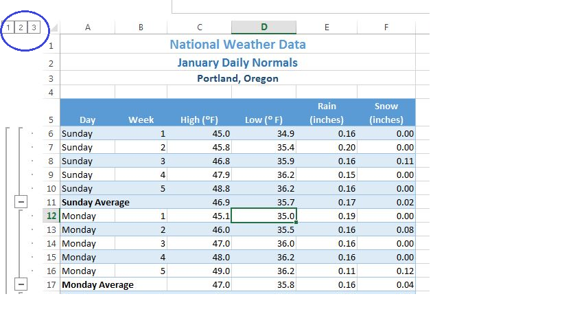
Notice the three Outline buttons circled in the upper-left corner of the spreadsheet. These allow you to control the amount of subtotaled data that is displayed. Table 5.5 describes the different Outline buttons.
Table 5.5 Subtotal Outline Buttons
| Button | Content Displayed |
| Level 1 | Only grand total
|
| Level 2 | Subtotals and grand total
|
| Level 3 | Individual records, subtotals, and grand total |
Let’s try the three Outline buttons to see the difference in the data displayed:
- Click on the 1 Outline button in the upper left-hand corner of the sheet.
- You should see only the Grand Average row with averages for High, Low, Rain, and Snow.
- Click on the 2 Outline button.
- Now you’ll see the average for each day of the week along with the Grand Average.
- Click on the + Sign button to the left of the Sunday Average row.
- This expands just the Sunday Day data and displays the individual records for this subset of the data. Clicking on + Sign buttons will expand a portion of the data at a time. Clicking on – Sign buttons hide a portion of the data at a time.
- Click on the 3 Outline button.
- All the individual records along with the subtotals, and Grand Average should be displayed.
- Save your Excel file.
Key Takeaways
- Filtering is an easy way to see a subset of your data. Filtering arrows appear to the right of each column heading when you insert a table with a header row.
- You can filter by text or numerically.
- A slicer is another way to filter in Excel that provides a set of filtering buttons on your sheet.
- Adding a total row to a table is a quick, efficient way to see summary statistics for one or more columns in a table.
- Subtotaling provides a way to quickly add totals to groups within a column along with providing a grand total at the bottom of the table.
- Subtotal Outline buttons allow users to see add of the subtotaled data, just the totals and grand total, or simply the grand total.
- Plus and minus buttons within subtotaling allow a user to expand and hide portions of the subtotaled data.
Attribution
“5.2 Intermediate Table Skills” by Diane Shingledecker, Portland Community College is licensed under CC BY 4.0
