
21 Artificial Intelligence
Introduction
Since the course has concentrated only on the PLC and Boolean logic, very little time has been spent on other types of programming architectures. Most processes are not deterministic and must have applied a number of different approaches for overall control. Some processes are very deterministic. For example, a sequencer sees a process as a sequence of numbers. Each number defines a state of the machine. Transferring a sequential operation to a sequence of numbers is easy to visualize (and program). Other programs may require a form of learning that may be programmed as part of the overall PLC program. As computer learning becomes more a part of the project, the decision should be made whether or not to use an artificial intelligence programming method (AI). Different types of AI will be discussed in this chapter as well as some mathematical modeling techniques that can aid in machine control.
Statistical forecasting methods used in modeling and forecasting serve to introduce the chapter.
After a look at statistical forecasting methods, an introduction to relational AI occurs. Relational AI is at the core of artificial intelligence programming. Introduced are early tests for machine thought processing as well as discussion of various types of machine intelligence. Questions of ethics and scope of use of AI are discussed as well. A problem using a search agent introduces the decision tree search algorithm. The problem introduced to searching a maze is useful throughout the chapter and becomes one of the few programs easily adapted to the PLC for implementation. More sophisticated search methods are also discussed although their implementation is not included. Probability is introduced as a means to choose a best path through a tree. The section on probability includes the development of Bayes’ Theorem and gives examples of its use. More sophisticated examples of problems solved by AI programs are given but not solved since they are not readily implemented in the programming of the standard PLC instruction set.
Knowledge-based expert systems must also consider fuzzy logic and neural network systems. Fuzzy logic deals with fuzzy linguistic terms while neural networks can learn using supervised and unsupervised learning. Once considered part of the core of modern AI, fuzzy logic and neural networks are not as popular as at one time and are not considered as a first solution in most AI problems.
Learning in the PLC
A PLC application that could be described as a program that learns in the PLC could include the example program requiring accurate closing a valve when the weight is being sensed. Some of the weight is in the air and not yet on the scale when the valve is closed. An amount of early cut-off must always be anticipated. However, as the vessel above the scale empties, the velocity of the liquid flow slows. The amount of weight that the valve shuts off may not only depend on a constant “pre-act” but also with the variation in the height of the material in the vessel. If it is important to control the weight on the scale exactly, then an adjustment must be made which is constantly finding a best model when the vessel is close to empty or close to full.
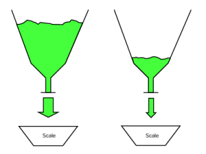
Fig. 21-1 Vessels Weighing onto Scale
In the figure above, the left vessel will empty at a slightly faster rate than the vessel on the right. The weight pushing down will not only cause a faster rate of flow but also change dynamically as the product empties from the vessel. This may create a need for an algorithm that is constantly hunting for a best pre-act weight to turn off the valve controlling flow from the vessel. While a hunting program may not imply an advanced learning algorithm, it can be seen that a form of a learning program must be employed. What happens to the algorithm when the vessel is refilled? What happens if the refilling occurs as the scale vessel is also being filled?
Statistical Methods in Forecasting
Statistical methods that model a process include a number of different analytical tools that can forecast an output depending on one or more input variables. Models can be used to predict and control a process more closely than other digital control methods if the model is a mathematical model of a process or a statistical model. One of these tools is statistical regression analysis. It is useful for predicting a statistical best fit for a new outcome based on past occurrences.
The regression equation is found by solving for the variables to satisfy the equation:
Y = a + b*X Eq. 21-1
In which the constant a is the y intercept and b is the slope of the line. If multiple X input variables exist, the equation becomes:
Y = a + b1*X1 + b2*X2 + … + bp*Xp Eq. 21-2
The variables for a and b1,b2,…,bp are found using the principles of least-square distances from each variable to the line generated. Finding these constants and then determining the best fit using only a small set of the entire set of input variables becomes a problem for this method. Also, determining whether the relationship is linear or other mathematical function is also important for a best fit of the data.
A more powerful tool called ARIMA is a good forecasting tool. ARIMA or AutoRegressive Integrated Moving Average is a tool for predicting future variables based on past occurrences of a number of different variables as well as the error of past occurrences based on the model. Included in ARIMA forecasting is the ability to introduce periodicity or a separate set of variables based on errors that are periodic over a cycle of time.
Regression analysis as well as ARIMA and other forecasting tools are available in a number of statistical packages such as MiniTab. Statistical packages have the ability to predict an outcome based on a number of different sets of existing data. Similar solution algorithms exist for the types of forecasting packages. Rules and rule writing are more a topic of the AI packages while the statistical packages offer a number of checking algorithms to get a best fit for the data used.
ARIMA(p,d,q)
ARIMA models are sometimes referred to as a random-walk or random-trend model for a variable or number of variables. The reference (p,d,q) identifies the number of regressive terms, difference terms, and lagged error terms in the model.
For a model of ARIMA(p,d,q) model:
- p = number of autoregressive terms
- d = number of differences
- q = number of lagged errors
For ARIMA(0,1,0), the equation for the model may be written:
Ŷ(t) – Y (t – 1) = µ Eq. 21-3
where Ŷ (t) º predicted value,
and
Y (t -1) = value at last reading
µ= a constant.
For ARIMA(1,1,0), the equation for the model may be written:
Ŷ (t) – Y (t -1) = µ + Φ(Y (t -1) – Y (t – 2) Eq. 21-4A
or:
Ŷ (t) = µ + Y (t – 1) + Φ(Y (t – 1) – Y (t – 2) Eq. 21-4B
where Φ = difference operation constant.
This equation is referred to as a first order autoregressive model. This is sometimes referenced as AR(1) or AR(1,1). As with any modeling process, the difficulty arises in finding the best sets of constants to precede each modeled variable and the number of the order of each variable. For instance, is AR(1,1,0) best or should AR(2,1,0) be used?
Each of these decisions is based on analytical results as well as the person modeling the data. An informed decision is to be chosen in each case. If seasonal data is present, then
the seasonal data must be accounted for in a separate variable. Next is an example of an ARIMA formula using only differencing and error-smoothing. This model is used to correct for errors with a periodicity over time.
ARIMA(0,1,1)
The equation for this model may be written:
Ŷ (t) = Y (t – 1) – Θ × e(t – 1) Eq. 21-5
where Θ = error operation constant
and e = error of the last reading.
With the error term, e(t-1) is the error at period (t-1). If multiple periods generate an error with periodicity, the error term might include more than one term such as ARIMA(0,1,2) or ARIMA(0,1,3). Rarely do terms including error terms extend more than 2 or 3 terms into the past.
Prediction of future values based on past values of a set of data is important for any kind of forecasting. The data generated is important in predicting a best case set of data for forecasting a set of data. While not able to predict unexpected occurrences or rational thought, such statistical methods as ARIMA are very useful in modeling a process.
The products of regression analysis or ARIMA forecasting can be used in a PLC program to build and analyze a model. Any model generation is done in a computer, however, usually with a good statistical package being used.
Introduction to Relational AI
Relational artificial intelligence can be viewed as a problem that seems to be more easily solved by humans than by computers. AI refers to those techniques that solve these problems through logic, probability, and other methods. The question of whether it refers more to science than to engineering may also be raised. In fact, it may be viewed as both. These systems may seem to think like a human. They may also be described as systems that act rationally or that may even “think” rationally. Most applications do not require the program to “think”, but rather only to behave rationally.
Thinking and Acting Rationally
The study of AI implies intelligence in the design of a program that is more than what has previously been discussed or available using Boolean logic and the other instructions of the PLC or computer. Obvious is the need to use logic to solve problems that are more difficult than can be solved using direct techniques. Most applications require sufficient knowledge to solve the problem at hand. If the information is not available, the use of a model or AI may bridge the area with insufficient knowledge to proceed otherwise. In any application, there is a trade-off between knowledge, cost of implementation and time to complete the project. Many times, there is not enough time to provide a logical decision but a decision must still be made. When this is the case, a rational decision is still necessary. Rational action may include a full set of facts but may not include all those facts. AI uses a rational approach to describe what is known. The use of rational agents is the best overall design approach. What is a rational agent? This will be considered throughout this section and includes programs that respond to a set of rules to provide a best answer to the problem at hand.
What is acting rationally? Implied in acting rationally is the concept of “doing the right thing.” Not necessarily implied is the idea of thinking. The goal of the problem is to be the primary consideration.
Not accepted are concepts such as irrationality or sanity or insanity. Also not considered is the concept that rational is equated to successful.
A rational agent is used to determine the success of a problem. The agent is a program in most cases that acts on the rules, considers the evidence and constraints, and provides a sufficient answer at each step to move forward to a succeeding step or sequence.
Most real world problems contain much uncertainty coupled with a great deal of complexity. Usually, the model or the program containing the model of the process approximates the process in a rational form. It has been said that a better title for any discussion of AI would be “computational rationality.” Thinking humanly implies thinking or getting inside the human mind. This is of little importance in this discussion.
Ethics and AI
Ethics and solving problems using AI or other principles should include asking some questions pertaining to the result of the application. For example, is it good or bad for the principles of AI to be used where someone might lose his or her job in the process?
Also to be considered is the issue of leisure time and the automation of the world around us. Should people have more leisure time as a result of using AI in automation?
Is there a problem with the sameness of a solution in which the human has little chance to show tendencies unique to his or her own personality? Also is the issue of personal privacy. Should the person be studied to make the process as efficient as possible and use the information from the process to further ask the individual to perform better?
On the other hand, if an AI system is implemented, do people tend to lose their sense of accountability and just give decision making over to the machine? Is this good or not? Is there a sense in which we as humans may lose some of our distinctive human qualities as a result of applying the principles of AI? I don’t necessarily believe this to be the case but each individual should ask these questions as he or she is programming a sophisticated project using principles of AI or modeling.
Quiz
Which of the following can be done at present?
- Can a program using AI play a movement game such as ping pong?
- Can a program using AI navigate a car along a twisting mountain road? How about navigating a car on Telegraph Rd?
- Could a program using AI buy a week’s worth of groceries at the local Kroger?
- Could a program using AI carry on a lively conversation about football with a person?
- Would you trust a program written with AI to perform a delicate surgery to your body? No, absolutely no.
- Translate a copy of a foreign language book to English.
- What can you add to this list of automation programs that you wish AI could do?
- What programs are you very satisfied that have not been automated?
What Can AI Do For You?
Some areas that use AI include language and speech recognition. Automatic speech recognition (ASR) has been around for many years and has been explored thoroughly. Other technologies such as text-to-speech synthesis (TTS) and dialog systems are available.
Language processing includes the easy translation such as:
Two plus two equals four.
Or the more difficult:
The program had a “jump the shark” effect.
The first is translatable into a second language easily but the second statement assumes knowledge of a television program used to over-state and thus drive viewers away. The specific example was the example of the Fonz on Happy Days who jumped a shark while water skiing. The program was commonly thought to be the program that convinced viewers that most possible scripts had been explored and nothing new was left to be explored. The “jump the shark” episode led to the loss of viewers to the program and its eventual cancellation by the network. Unless the translator knew the meaning of “jump the shark”, the translation would have little hope of a proper translation.
Computer operating systems include such AI programs as information extraction and retrieval, question answering, spam filtering and spell-check. Vision systems furnish a number of very difficult questions for any program and may turn to AI for perception and recognition of a part. Robotics includes elements of AI as well as mechanical engineering. Both the mechanical arm and the movement of that arm are included in the programmed movement of the robot. Simulations only provide a portion of the final answer and most robotic applications must be run in realtime with real mechanical equipment to find answers concerning the practicality of the robot.
Technologies such as movement in a confined space, rescue vehicles, vehicles capable of movement in a contaminated environment, capable of movement in a combat environment are common to those in robotics. Systems using logic to prove various other math concepts or principles may be found in AI. NASA even uses AI at times in their fault analysis and diagnostic routines.
Do not forget the use of AI in such game playing as chess. Deep Blue is a computer program known to play and defeat the most adept chess player. The question should be how any human can compete with a computer in competitions involving such complex games as chess. Man has defeated the computer for many years but in the last decade, the computer has become more complete in assessing the complexity of the game and been able to dominate the man in most cases.
Most processes or problems dealt with in AI and in general are stochastic rather than deterministic. That is, most processes are not known in their entirety and must be dealt with from an imperfect model. No model can be constructed that perfectly determines each output based on each input.
Search Problem: Moving Through a Maze
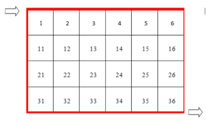
A task that can be programmed using the PLC is the following project. It consists of an arrow or agent moving through a maze. Rules for movement may vary depending on the complexity of the maze. The following maze includes an entry point and an exit point that is fixed. Walls inside the maze may be installed at any segment.
Fig. 21-2
Cells must be numbered to be identified for use in the program. For instance, an arrow moving from cell 1 may only move to cell 2 or 11 if wall segments do not block movement of the arrow from cell 1. The following shows the maze with each cell numbered to identify movement in the maze.
Fig. 21-3
A method must be provided for inclusion of walls for the maze. If a wall segment is installed, the graphic picture of the maze should include the blocking segment and the program should include a 1 adjacent to that wall segment. Edges block the movement unless the edge segment allows the arrow movement into the puzzle or out of the puzzle. Cells 1 and 36 are used for this action.
IMAGE
The following puzzle gives an example of the maze with walls and sides installed. Movement through the maze would be implemented with the sequence:
In-1, 1-11, 11-12, 12-22, 22-32, 32-33, 33-23, 23-13, 13-14, 14-24, 24-25, 25-15, 15-5, 5-6, 6-16, 16-26, 26-36 and 36-Out
Fig. 21-4
The maze can be represented as a state graph in which nodes become the states, arcs are actions and arc weights provide a cost of movement from state to state.
Fig. 21-5 State Graph with Arcs
The program must be designed to move through the states or nodes in a smart way. If weights are considered, it is important to keep weights updated as the program moves forward.
If a table of historical events is saved, the table may grow quickly to a very large size. The user may be faced with an impossible program to write to keep track of all the historical information.
Cell 13 presents the algorithm of which cell to explore first, either cell 12, 3 or 14. These cells must be known as the cells to explore. Information about walls and sides and historical information of prior cell movement must also be included in the decision- making process.
Fig. 21-6 Movement from Cell 23 to Cell 13
Fig 21-7 Movement in Cell 13
First, add to stack the last node address, in this case, 23. Then a choice must be made how to proceed. The following choices are available:
12, 3, or 14
| 12: | No | |
| 3: | Yes | Has this square been explored before |
| 14: | Yes | Has this square been explored before |
Which one should be chosen? A decision must be made whether to provide equal weights between the various choices or weight the choice.
What happens if the arrow goes into a dead end? The arrow must depend on the stack to retrace its steps to a new un-explored square.
Fig. 21-8 A Dead End at 21
In the search algorithm for a next cell or square, a program or agent program must evaluate and return an action for movement forward through the maze or move backward to a former cell or give up. A set of inputs or percepts return and give a description of the present state. Initially null, the state has been updated with movement through the maze to this point. The problem defines a set of rules for making a decision based on these percepts and earlier states. The following table from the text gives a more formal description of this sequence. Be aware that the programming statements may be viewed as executing one or more of the following:
The search through the maze is an example of a search tree. The search tree may represent a number of paths through a state graph. Such search paths grow much larger than the state graph, however.
Each node may be described by the following five components:
- Present state
- Past or parent state or node
- Present action
- Cost of each path
- Depth into the tree
Consider whether a problem uses states or nodes is based on the fact that a problem graph consists of problem states with successor states and step cost while search trees consist of search nodes with parent and children nodes. Consideration must be given for depth in the tree, path through the tree, path cost and other considerations. While the present problem uses states and successor states, a close analogy exists with problems using the search tree method and its nodes.
As the rational agent moves through the maze, a stack is constructed that remembers how to move backwards to a second acceptable path if the present path is blocked. In general, the fringe references those states or nodes not explored but passed by as the agent moves through the maze.
The stack keeps track of the path the rational agent moves through the puzzle using the rational agent program. A stack may act to states of empty, first state, next state or last state. In a stack, a sequence of steps is saved which may be retrieved to satisfy the algorithm’s need to back up and try another step or to conclude a search either with a successful result or an unsuccessful end.
The problem must either find a solution or end in failure. The program must measure success toward the solution. If a solution is not reached and the stack is finally exhausted (emptied), then no solution exists.
Fig. 21-9 Stack Representing Present Path
An important problem to be considered in AI is the search for a sequence of nodes or states that maximize performance in future steps. This may include planning or other search algorithms. Also, it is important to search for future consequences of present step actions. It is also important to consider a model that might fit the algorithm. Any insight that might lead to a solution is acceptable to insert in the algorithm for possible inclusion in the overall program. Search techniques such as those to solve the maze or other node problem were some of the early successes of early AI research.
Simplest of the agent programs are the reflex agent programs. With these programs, there is a direct mapping from states to actions. These programs do not operate well where there is a demand for large amounts of memory storage or a large amount of time to learn a possible algorithm or solve the puzzle. Goal-based agents are unlike reflex agents in that they can succeed by considering future actions and making decisions about desirability of these decisions. These are called problem-solving agents. They decide what to do by finding sequences of actions that lead to desirable states as the program proceeds. The algorithms are uninformed in the sense that they are given no information about the problem other than its definition. A path cost function may be included that assigns a numeric cost to each path.
Other Problems Using Reflex or Goal-Based Agents
Each problem has a unique set of conditions that define a constraint satisfaction problem. For the goal of any problem to be successfully achieved, a set of constraints specifying combinations of values must be satisfied.
Cryptarithmetic Puzzles
The letters S, E, N, D, M, O, R, Y are digits that are unique from each other. They (SEND + MORE ) may be added together and equal the result represent MONEY. None of the numbers may begin with zero. This may be represented as follows:
S E N D
+ M O R E
– – – – – – – – – – – – – – –
M O N E Y
The following relationships apply for the letters and their possible numeric equivalents.
S : : 0 . . 9, E : : 0 . . 9, N : : 0 . . 9, D : : 0 . . 9,
M : : 0 . . 9, O : : 0 . . 9, R : : 0 . . 9, Y : : 0 . . 9, Eq. 21-6
Also,
S >= 1, M >= 1
The following algebraic condition holds:
S * 1000 + E * 100 + N * 10 + D
+ M * 1000 + O * 100 + R * 10 + E
= M * 10000 + O * 1000 + N * 100 + E * 10 + Y Eq. 21-7
Uniqueness requires the following:
S != E, S != N, S != D, S != M, …
E != N, E != D, E != M, …
N != D, N != M, …
…. Eq. 21-8
The problem is to find the numeric values of S, E, N, D, M, O, R, Y. This problem is most easily solved using a procedural language such as C instead of a PLC program although the looping instructions of the PLC make the procedure easier than for those PLCs without iterative looping.
8-Puzzle
Starting with a start state such as the one shown below, move the squares similarly to the sliding puzzle game and find a solution that moves the tiles to the finish state shown below:
Start State Finish State
Create an appropriate state model describing the actions needed to move a tile.
Next is a sequence of states for the 8-puzzle problem. The solution for this puzzle may be found by expanding the possible states until a solution is found at a specific state.
For the 8-Puzzle problem, each of the moves of 5, 4, 6, and 2 to the center must be considered before any second moves are considered. This may be advantageous in some problems but probably not here.
Fig. 21-10
This is an example of a program that can repeat to an earlier state, a problem that must be avoided. The BFS search continues with each state evaluating to more states from each prior state until the finish state is achieved.
Real-world Problems
Example: Assembly in an automotive or other manufacturing facility
Questions such as what states comprise the set of acceptable states the process must move through. What is the ultimate goal of the manufacturing process? What actions are needed to accomplish the task? What are the associated costs with the various aspects of the manufacturing action? All these questions need to be answered to successfully accomplish the goal of the company.
Tree Search
A tree search is the basic mechanism for the problems discussed in this portion of AI. Graph problems as well as a number of node-defined programs are included in the mix of problems addressed by tree searches.
The tree search may be visually described as a tree with many branches and choices from branch to branch through the tree. Viewed as a decision tree, the following shows the possible solution paths:
Fig. 21-11 Tree for Search Tree Problems
In this tree, the path starts at 1, then to either a or b, and then to a1, a2, a3, b1, b2, or b3. The program moves from node to node along a path with the active path or paths along a line referred to as the fringe. If the fringe becomes empty, the problem is complete. The fringe defines the possible next locations the program can be active in.
Each node leads to a new set of nodes which are then to be evaluated. The parent node is the node that other nodes branch from. Path costs may be used to determine a preferred path. Path costs are either determined before the program begins or as the program progresses.
Uninformed Search Strategies
Depth First Search (DFS)
One of the tree uninformed search strategies is the depth first search. It may succeed in finding a least cost solution if one exists. It may become tied in an infinite path if path checking is not included. The variables for the Depth First Search include the following:
| n | Number of states in the problem |
| b | The average branching factor B
(the average number of successors) |
| C* | Cost of least cost solution |
| d | Depth of the closest solution |
| m | Max depth of the search tree |
Definitions of Depth First Search Variables
Depth first search implies the search of a particular path with a cost advantage followed from first step through to the last step. If the path doesn’t yield a successful answer, then a second, third, fourth, etc. path is followed until all paths are exhausted or no path is found to satisfy conditions of the problem.
Fig. 21-12 Path of Depth First Search
Breadth First Search (BFS)
The second uninformed search strategy is breadth first search. Breadth first considers each possible step and then each possible second step resulting from a first step. This method grows to include a great deal of memory and may become unwieldy if not carefully crafted in its planning. There are some problems for which BFS will outperform DFS and vice versa. If repeated steps are not deleted and carefully screened out of the problem, successive steps may be repeated inadvertently. This will create much more work for the program than would otherwise be required.
Fig. 21-13 Paths of Breadth First Search
Graph Search Problems
A graph problem similar to the graph shown below is a special type of tree problem. Graph problems may be represented by the matrix A[i][j] below and are used to explore problems such as the traveling salesman problem. In the traveling salesman problem, the object is to find a route of minimum length that allows the salesman to visit all cities in his route only once. The graphic method contains edges or connectors between objects or states. If a connector has an arrow, the path is directed and can only occur in the direction of the arrow. Graph problems are rather simple and require an algorithm in addition to the array and a table of states already visited.
Graph Search Diagram and A[i][j] Matrix
| A[i][j] | 0 | 1 | 2 | 3 |
| 0 | 0 | 1 | 1 | 0 |
| 1 | 1 | 0 | 1 | 1 |
| 2 | 1 | 1 | 0 | 1 |
| 3 | 0 | 1 | 1 | 0 |
If the graph edges are directed (arrow pointing in one direction only), the matrix only reflects the direction allowed. For example,the path from 0 to 1 is directed. The array reflects the path direction by placing a 1 in the A[0,1] element and placing a 0 in the A[0,1] element.
Graph Search Directed Diagram and A[i][j] Matrix
Numbers other than 1 can be used to represent weights in the graph. For example, if the cost of going between 0 and 1 was 10, the weight 10 would replace the matrix location of A[0,1].
| A[i][j] | 0 | 1 | 2 | 3 |
| 0 | 0 | 1 | 1 | 0 |
| 1 | 0 | 0 | 0 | 1 |
| 2 | 1 | 1 | 0 | 1 |
| 3 | 0 | 1 | 1 | 0 |
Special Types of BFS and DFS
Graph Search
A problem of finding a best route through a series of cities to a destination is the object of a graph search problem. For the graph search problem, the BFS technique is used with the added criterion that a node is never expanded twice. For a graph search algorithm to find the answer each possible solution is found and a best one is determined based on the route criteria. The criteria should include miles traveled or time to travel the route or a combination of the two. Other rules may include delays for construction. Programs such as MapQuest and other web directions programs incorporate these program elements.
Iterative Deepening
Iterative deepening uses DFS as a subroutine and solves an algorithm with weighted lengths that are below a threshold. First the lowest threshold is searched (assumed = 1) followed by higher thresholds (2, 3, and higher). The BFS algorithm finds a solution using the least number of transitions while the iterative deepening algorithm expands the algorithm to include a least-cost path. Other algorithms expand these concepts.
Uniform Cost Search
This algorithm expands the cheapest node first while keeping the fringe a priority queue.
Priority Queue Refresher
This algorithm stores a pair (key, value) for each state. As a state is evaluated, keys may be promoted or demoted by resetting key priority. The result is a priority queue. Priority queues are used in finding solutions for most cost sensitive algorithms involved in search.
More Problems for BFS and DFS
- Find a method to evaluate a planar map with only four colors. The only criterion is that no two adjacent regions have the same color. Find if no solution exists. This problem requires backtracking as a search method.
- A three foot tall monkey with a total four foot reach is in a room with bananas suspended at 9 ft from the floor. He can access two 3-ft tall crates. Describe how the monkey can access the bananas.
- There are three jugs in your garage of size 12 gallons, 8 gallons and 3 gallons. You have access to a water faucet. Find a procedure to measure one gallon of water. You may pour water from one jug to another or dump the water on the ground.
- Three missionaries and three cannibals are present on the west side of the river. There exists a canoe capable of transporting one or two people at a time across the river. Formulate a series of steps to move the missionaries safely to the east side of the river. Did I forget to mention that any imbalance in the number of missionaries and cannibals in favor of the cannibals will result in instant doom for the poor missionaries.
Fig. 21-14 Missionary and Cannibal Puzzle Layout
Cracker Barrel 15-Hole Puzzle
One description of this game describes its ease of solution on a computer due to its small size. Two solutions are shown below. Find a solution to this solitaire game using a computer solution.
Solutions are similar to one of the two solutions below:
Fig. 21-15 Layout of Cracker Barrel 15-Hole Puzzle
Informed (Heuristic) Search Strategies
A heuristic is assumed to include an estimated distance to a particular goal. It involves some information deduced by a strategy that is informed rather than uninformed.
Included in heuristic strategies are a number of different search methods including
- Best First Search
- Greedy Best-First Search
- Uniform-Cost Search (UCS)
- Combined UCS and Greedy
Each of these search methods can be lumped into a general heuristic search method commonly referred to as A*.
An example of an informed search could include course scheduling. It may be ordered from the perspective of the university, a search problem definition and known heuristics. For example, the university controls the set of courses, the availability of class rooms, possible pairings of classes with rooms and a list of what classes fit best in what rooms. The result is a cost of pairings that optimally finds a best fit for each class offered and a set of rooms.
Multi-Player Games
These games may be two-player or multiple player games. The game tic-tac-toe is used as an example and the search algorithm is referred to as mini-max in which one player maximizes the result and the second player minimizes the result.
In the mini-max game strategy, as a play is executed, a resulting set of solutions is calculated. The starting grid may have nine possible entries followed by eight possible entries, then seven, six, etc. A terminal solution may be reached any time one player wins or the grid is filled. The value is -1 if player 1 is winner while +1 if player 2 is winner.
Fig. 21-16 Tic-Tac-Toe Path to Solution
A process referred to as pruning in the minimax search encourages the program to proceed along paths or configurations in order to win. If a path leads to a loss, prune or get rid of that branch.
In order to determine a path, a probability may be attached to that path. Those not using probability are referred to as deterministic while those using probability are referred to as probabilistic models. Problems may also be referred to as propositional or relational.
Introduction to Probability
Probability Theory
To determine whether an action will take place or not, a probability is usually assigned to
the action. For example, let the action At be the probability that if I leave for the airport t minutes before a flight, will I get on the plane? In other words, will At get me there on time?
Most problems contain some uncertainty. The problem may be only partially observable or contain noisy sensors. Unexpected events may occur during the process. Also, the machine or decision process may incorporate so sophisticated a set of rules that no good model exists by which to predict an outcome. With any of these problems, probability is a good approach to determine outcomes.
With a purely logic approach and the example of getting to the plane on time, a logical approach will be either an absolute “yes” answer or “no” with no room for comparing probabilities and choosing a best path. The possibility that a good decision is going to be made varies with each of the factors listed above and these factors may be dynamic and not completely observable. On the way to the airport, a semi might decide to turn over, a completely unexpected event, with catastrophic results pertinent to getting to a plane.
It is easier to say the following:
“A80 is ok to get me to the airport on time”
It is more powerful to say the following:
“A80 will get me there on time if there are no accidents and the weather is fine and my automobile doesn’t have a flat tire, etc.”
For those of us with low tolerance for failure, it might be more comforting to say:
“A1440 will be fine for getting me to the airport. But, for safety and comfort, I will need to check in at the airport hotel the night before to insure my flight.”
Using probability, it is possible to write probability for each of the time choices for going to the airport.
For example, with no further information, A80 can get me there successfully with a probability 0.6. (The probability of 1.0 is perfect guaranteeing the desired result.) The probability of getting to the airport in 80 minutes can be written:
P(A80 ) = 0.6
The probability of getting to the airport can change with new evidence. For example, any of the following can add some information and give the probability a higher probability or lower probability:
P(A80 | 5am) = 0.8
P(A80 | 5am) = 0.5
P(A80 | accident report, 5am) = 0.3
P(A80 | accident report) = 0.1
In general, new information gives a better picture of the overall situation allowing an informed decision-maker input as to whether or not to get in his or her car and make the trip to the airport. The more one listens to accident and weather reports, the more one is informed as to the chance that a trip to the airport will succeed. At some point, most people make a decision and adjust future decisions based on the history of whether past trips were successful. If a trip did not succeed, the appropriate action taken to correct the problem is a high priority to most people since missing an airplane causes a great deal of upset to most people. To the well-traveled professional, the level of upset is minimal.
They calculate that there will be another plane and they will take it. They have done this before with little disruption to their lives. Most people, on the other hand, would do whatever it takes to guarantee success on the trip at hand. They would expect and do whatever was necessary to guarantee success with this trip.
The probabilistic model generated from this simple decision gives more information from which to make an informed decision. As part of a decision tree problem, probabilistic models give information about which branch to travel first, second, third. The probability information contained can also be upgraded or adjusted with outcomes that change the overall problem.
Example: Warm and Sunny
Probabilistic models are created from conditions that give a description of the problem at hand. For example, in the description below, it is either warm or cold and sunny or rainy.
The total probability of each occurrence is assigned a probability with the total normalized to 1.0. The probability that it is warn and sunny is .4, warm and rainy, .1, cold and sunny, .2, and cold and rainy, .3. In table format, the description would be:
| A | B | Probability |
| warm | sunny | 0.4 |
| warm | rainy | 0.1 |
| cold | sunny | 0.2 |
| cold | rainy | 0.3 |
Fig. 21-17 Probability for Warm/Cold and Sunny/Rainy
Probabilities are seen as averages over a number of repeated observations or experiments. The observations may have occurred over a number of years or just a short period of time but must have enough samples to constitute a valid sample. One or two observations do not constitute a probability. The number of samples that is sufficient to provide an adequate sample is called the confidence interval.
Even variables over which no observations have occurred have probabilities. They are not assigned because we do not know what they are.
We use probabilities for a wide range of activities, not just for games of chance. For instance, if I am feverish, am I sick? If an email contains a reference to “Viagra”, is it an example of spam? A probability could be attached to whether a person should get up or not in the morning based on a meteor hitting them. Usually, these probabilities are rather small.
Some processes are inherently random. Tossing of dice falls into this category (unless the dice are weighted). Sometimes a variable may not be known and is therefore, not included in a program. This and many other problems cause uncertainty in a process.
While fuzzy logic may define certain variables in a new way, the difference between fuzzy logic and the probability assignments in this section are separate topics.
Mathematically, a distribution can be described as a joint distribution over a set of random variables. A joint distribution over a set of random variables X1, X2, . . . , Xn, is a map from assignments to reals. It may be defined as:
P( X 1 = x1 , X 2 = x2 ,…, X n = xn )
P(x1, x2 ,…, xn ) Eq. 21-11
The probabilities of these variables must obey the following:
o≤ P(x1 , x2 ,…, xn)≤1
Σ(x1 , x2 ,…, xn) P(x1 , x2 ,…, xn) =1 Eq. 21-12
An event can be defined as a set of assignments (defined as E):
P(E) = Σ( x1 , x2 ,…, xn )∈E P(x1 , x2 ,…, xn ) Eq. 21-13
Eq. 13-12 and Table 13-4 confirm that the probability of all occurrences add to 1. In Table 13-5, a third variable, summer/winter, is added to the table above. This would indicate additional information from which to make a decision. Joint distributions are the sum of several events. The table below can be used to calculate joint distributions using Eq. 13-13 and the table. For example, it is possible to calculate the probability that it is warm AND sunny, probability that it is warm, or the probability that it is warm OR sunny.
Add Summer/Winter to Example
The table below gives the combined warm/cold, sun/rain and summer/winter probability for the example of summer/winter, warm/cold and sun/rain:
| S | T | R | P |
| summer | warm | sun | 0.30 |
| summer | warm | rain | 0.05 |
| summer | cold | sun | 0.10 |
| summer | cold | rain | 0.05 |
| winter | warm | sun | 0.10 |
| winter | warm | rain | 0.05 |
| winter | cold | sun | 0.15 |
| winter | cold | rain | 0.20 |
Sum =1.00
Fig. 21-18 Probability for Warm/Cold, Sunny/Rainy, and Summer/Winter
Probabilities can be written in the following way:
P(S=w, T=w, R=r)
For example, the first is the probability of the season being winter. The second is the probability of the temperature being warm. The third is the probability of the weather being rain.
The following table shows the probability of the temperature being warm or cold:
P(T)=
| T | P |
| warm | 0.5 |
| cold | 0.5 |
The following table shows the probability of the weather being sun or rain:
P(R)=
| R | P |
| sun | 0.65 |
| rain | 0.35 |
The following table shows the probability of summer or winter, warm or cold:
P(S,T)=
| S | T | P |
| summer | warm | 0.35 |
| summer | cold | 0.15 |
| winter | warm | 0.15 |
| winter | cold | 0.35 |
The combined probabilities at the right are referred to as the marginalized value for the joint distribution over a subset of the total number of variables.
Conditional Probability
A conditional probability is the probability of an event given another event (evidence). It is described as:
P(a | b) = P(a, b)
P(b) Eq. 21-14
and is read as the following:
”the probability of a given that b occurred is the probability of a and b divided by the probability of b.”
The probability of a and b can be described as the intersection of a and b in the following figure:
Fig. 21-19 Intersection of a and b or P(a,b)
Examples of Conditional Probabilities
The probability of temperature and rain together can be described:
P(T, R)
In table form, the probabilities of temperature and rain are described:
| T | R | P |
| warm | sun | 0.4 |
| warm | rain | 0.1 |
| cold | sun | 0.2 |
| cold | rain | 0.3 |
Use the table to describe the probability of rain given that it is cold, written P(r|c):
Use Eq. 21-14 to describe the calculated probability:
P(r | c) = P(c, r)
P(c) ( Eq. 21-14)
or
P(r | c) = 0.3
0.5
or 0.6
Conditional probabilities are also known as posterior probabilities. If the conditional or posterior probability is all that is known, Eq. 21-14 can be used to calculate the other probabilities in the equation. For example:
P(cavity|toothache) = 0.8
This may be read “the probability that I have a cavity given that I have a toothache”.
The probability that there is a cavity and a toothache is described as the intersect:
P(cavity, toothache)
If this probability is known, then the probability that there is a toothache can be calculated.
P(cavity|toothache) = P(cavity, toothache)
P(cavity)
or
P(cavity) = P(cavity, toothache)
P(cavity|toothache)
If the probability of a toothache is known, then the probability that there is a cavity toothache can be calculated.
In general, if any two of the three parts of the formula is known, the third can be calculated.
Next, use the table discussed before to discuss more conditional probabilities:
| S | T | R | P |
| summer | warm | sun | 0.30 |
| summer | warm | rain | 0.05 |
| summer | cold | sun | 0.10 |
| summer | cold | rain | 0.05 |
| winter | warm | sun | 0.10 |
| winter | warm | rain | 0.05 |
| winter | cold | sun | 0.15 |
| winter | cold | rain | 0.20 |
Fig. 21-20 Probability for Warm/Cold, Sunny/Rainy, and Summer/Winter
The intersection of temperature = warm, rain = rain and season = summer is 0.05. This can be used to describe the probability of warm and rain given summer as the season. See the following calculations to prove this statement:
P(T = w, R = r | S = s)
= P(T = w, R = r, S = s)
P(S = s)
= 0.05 = 0.10
0.50
This can be described as:
P(T , R | S = s)
or
P(T , R | S )
Conditioning is fixing some variables and renormalizing over the rest:
P( X1 , X3| x2 ) =P( X1 , X2 , X3 )
Σx1 ,…, x3) P(x1 , x2, ,x3) Eq. 21-15
P( X1 , X3| x2 ) = P( X1 , X2 , X3 )
P(x2)
Sometimes joint P(X,Y) is easy to get while at other times the conditional probability P(X|Y) is easier to obtain.
Two variables are independent if and only if:
P(X,Y)=P(X)P(Y) Eq. 21-16
Independence is a modeling assumption and should always be considered when applying Eq. 21-15
With some probabilities, independence is assumed even though empirical evidence may no be exact. For example, one may toss a coin 100 times with the outcome of 70 heads and 30 tails. It may be assumed from the evidence that 70% heads and 30% tails is an acceptable probability but it is generally accepted that the probability for heads and tails is equal at 50%. This may be written as follows:
N fair, independent coins:
P(X1)
| H | .5 |
| T | .5 |
P(X2)
| H | .5 |
| T | .5 |
P(Xn)
| H | .5 |
| T | .5 |
or P(X1, X2,…, Xn,)=1/2n
If two variables are independent, the following can also be written for their joint distributions:
P(x | y)P( y) = P( y | x)P(x) Eq. 21-17
Dividing, we get:
P(x | y) = P( y | x)P(x)
P( y) Eq. 21-18a
This simple equation forms the basis for decision making of all modern AI programs and is known as Bayes’ rule.
This rule may be generalized to be written as the following:
P(Cause | Effect ) = P(Effect | Cause)P(Cause)
P(Effect ) Eq. 21-18b
Bayes’ rule can be used to describe a forward or backward movement through a tree structure. Additional statistical methods including maximum likelihood, Markov chains and other methods are used in cooperation with Bayes’ rule to complete the design of the search algorithm.
Bayesian networks are used to describe complex joint models using a group of simple distributions. They solve the problem of large joint probability distributions. Models are used to describe the probability model. The following figure shows a simple Bayes network ready to be evaluated.
Fig. 21-21 Example Bayes Network
A Bayes Network may be either independent or independent of prior nodes. For example, to say X and Z are independent would require that X does not influence Z. If this can be said, then the two are independent.
Fig. 21-22 Example Bayes Causal Chain
If Z is independent of X, then the effect of Y blocks the influence of X onto Z. This can be proven with the following formula using the Bayes Equation:
P(z | x, y) = P(x, y, z) =P(x)P( y | x)P(z | y)
P(x, y) P(x)P( y | x) Eq. 21-19
= P(z | y)
Another configuration of two effects that possibly influence each other is found below:
Fig. 21-23 Two Effects of Same Cause
Again, Y is common to both X and Z but X and Z do not affect each other. The proof is similar to the proof of the causal chain proof.
A third configuration shows two causes and a single effect. In this example, the question of independence of X and Z is no. They both influence the effect Y.
Fig. 21-24 Two Causes of Same Effect
Next to be discussed are two methods of analyzing or modeling a process using languages suited for learning a best response. They are neural networks and fuzzy logic. They are considered traditional approaches to problems in AI but are not as flexible as the general methods discussed in this section.
Process Simulation Software using Statistics
Statistical programs are not confined to AI. The following two programs give access to modeling of manufacturing processes. Studies can show without actually building the process whether there will be bottle-necks, whether flow will be interrupted and slowed. Each of these programs is based on statistical data generated from real processes and then fed into the model to predict how the new process will react.
First is Arena – a software package by Rockwell (Allen-Bradley) Rockwell describes the package as:
“Simulation software is the creation of a digital twin using historical data and vetted against your system’s actual results. Arena™ Simulation Software uses the discrete event method for most simulation efforts, but you will see in using the tool that we cover areas in flow and agent-based modeling as well.”
A tutorial on its use is found at:
https://nitc.ac.in/app/webroot/img/upload/Manual%20of%20SIMULATION%20WITH%20ARENA %20FOR%20LAB%20 %20Note.pdf
Arena software may be downloaded for free for students. It may be downloaded at the following site:
Siemens likewise offers a package – Tecnomatix Plant Simulation software.
“Tecnomatix Plant Simulation is 3D, object-oriented, discrete event simulation software that allows you to model, simulate, explore and optimize logistics systems and their processes. These models enable analysis of material flow, resource utilization and logistics for all levels of manufacturing planning from global production facilities to local plants and specific lines, well in advance of production execution.”
“STUDENTS! Please download a special student version of Plant Simulation software. It is very important that you follow this link and register to receive your software.
https://www.plm.automation.siemens.com/plmapp/education/plant-simulation/en_us/free- software/student”
A tutorial for the Siemens platform:
Simulation Modelling using Practical Examples:
A Plant Simulation Tutorial
While the topic of manufacturing simulation software may not have the interest of the student interested in automation, it possibly should be. These software packages represent a method of simulating the process to identify potential bottlenecks and other process problems. It may give important information as to what actually will be programmed and how the operator may access the information in the system. If an operator can mess up the process, they will. Guaranteed.
So, design of a process may many times depend on your set of parameters that the operator will be allowed to access and where they can access these parameters. If there is one possible location, the gatekeeper for that location is an extremely important person. If the process is spread out, then many gatekeepers may be present and can impede or thwart the wishes of another. Remember also that operators may be only on the job for a day or two before being asked to monitor and maintain important machines.
If you have ever seen a traffic jam (think New York City at rush hour or when an important dignitary is visiting), you have an idea as to what can happen when a process has several competing demands placed on it with only a few paths through it. There can be complete back-up of a system just as there is in a traffic jam. The traffic jam can be predicted with a good model and a good model can point to paths to better control the process.
Expert Systems
After looking at a number of learning and forecasting approaches to programs that may adapt or learn as they are executed, it is important to look at expert systems. First it is important to understand how people reason and then look at ways the computer can be adapted to use similar methods.
People reason first by creating categories. They sort things into these categories where it is easier to deal with the item or items than together.
They use rules to sort and categorize items. Included in the rules for a system may be boolean if/then statements as well as heuristic rules. Heuristic rules are commonly referred to as “rules of thumb”. Care must be taken to fully scrutinize these “rules of thumb” to not include ideas that are assumptions with no or little statistical data to back the heuristic. In general, heuristic data represents what is referred to as conventional wisdom.
People also use past experience which may seem similar to heuristics but also include “case histories”. They also use a set of expectations based on past observations. This may include an observation about past activity as well as general patterns of behavior.
How then do computers Reason? They are programmed by humans and carry the same sets of rules that people use. Computer modeling uses models based on human reasoning including frames, rules, cases and pattern recognition. Frame attributes may be referred to as slots. Rules include Boolean logic as well as knowledge-based rules. Pattern recognition includes voice/face recognition as well as database constructions to support the recognition programs.
Rule Based Reasoning is a form of expert system that includes a user interface, database, and inference engine as well as rules stored in a knowledge base.
Knowledge engineering includes various components. First is the process of knowledge acquisition and knowledge representation. Case-based reasoning also is included in this discipline of expert systems.
Neural Networks
Neural network programs are based on pattern recognition. They provide a set of simple mathematical elements using adjustable weights to produce output values. These adjustable weight patterns are able to sort through a large amount of noisy, ambiguous data and make sense of it when most systems cannot.
Neural networks use a method of training requiring feed-forward and feed-back propagation. How the layers of neurons are structured and the layers of hidden neurons included may vary from process to process with most systems having a favored group of layers for the particular process.
The neurons are the processing elements of the system. These neurons are based on the neuron in the brain and act in somewhat the same manner.
Since the course is primarily interested in processes that include machines, it is important to view neural networks from the vantage of how can neural networks be used to control or enhance machine logic. Machine learning as a part of neural networks also plays an important part in neural network control. The learning of a pattern such as a vision system that must identify a good or bad part as it is moving down a conveyor is an example of a learned process possibly using neural networks.
It is very hard to write a program in a PLC to recognize a face and identify it from all other faces. Even if such a program could be written, its complexity would be very great. Then if the face were to change in some way, to devise a learning program to adjust the algorithms would again require more time and effort. Even recognition of a writing sample carries many of the same problems of recognition of one letter or another. Some tasks are best solved using neural network’s learning algorithms.
One of the basic similarities between the brain and the use of neural networks centers on the idea of modularity. The brain can differentiate between different actions and compartmentalize these actions to various parts of the brain. The neural net program must be built to also compartmentalize and sort data for use. This task is crucial to a successful implementation.
Some learning networks deal with perceptron output and others deal with linear networks. Perceptron outputs are hard-limited to either 0 or 1 based on certain criteria in the network.
From MathWork’s Neural Network Toolbox,
“In this chapter, we design an adaptive linear system that responds to changes in its environment as it is operating. Linear networks that are adjusted at each time step based on new input and target vectors can find weights and biases that minimize the network’s sum-squared error for recent input and target vectors. Networks of this sort are often used in error cancellation, signal processing, and control systems.
The pioneering work in this field was done by Widrow and Hoff, who gave the name ADALINE to adaptive linear elements. The basic reference on this subject is: Widrow B. and S. D. Sterns, Adaptive Signal Processing, New York: Prentice-Hall 1985.”
Shown below are neuron types without and with bias.
Fig. 21-25 Neuron without Bias
In the above: p = input to neuron
a = f(wp)
image
In the above: p = input to neuron
a = f(wp + b)
The figure below gives a neuron with vector input. R is the number of elements in the input vector. In this example, the output a can be expressed as:
A=f(Wp + b) Eq. 21-20
Neuron with Vector Input
As a layer of neurons is combined with the same input vector, the following figure would be found:
Fig. 21-26 A Single Layer of Neurons
S is the number of neurons in the layer. For one layer, the vector equation
a = f(Wp + b)
is used. Eq. 21-21
If more than one layer is added, the following is implemented:
Fig. 21-27 A Three Layer Group of Neurons
As can be seen, values of the a vector for early layers are fed as input to the later layers. These layers use the input from the earlier layer and output a new a value based on the neurons in the layer
Transfer functions vary and may include the following two examples:
Fig. 21-28 Linear Transfer Function
The equation for the linear transfer function is a = purelin(n).
Fig. 21-29 Linear Transfer Function
Example of Neurnal Network
w = (wburger wfries , wsoda ) Eq. 21-22
You go to the same fast food drive-through for lunch each day and order the same three items – a burger, fries and a soda. One day you may buy 1 burger but the next day you may be hungrier and buy 2 or 3. Likewise, you order any number of orders of fries or sodas. The cashier only gives back change and never tells the value of the three individual items. You log the price each day of the total amount spent.
Over time, you have a number of different prices that you may refer to as “price” and you should be able to calculate the price of each item in the meal. The process to find each price may be simpler using algebra or possibly even regression analysis but for this example, we will use the neural network to approximate the price of each item.
price = x fishwfish + xchipswchips + xbeerwbeer Eq. 21-23
What is desired are the values of the three weights as follows:
w = (wburger , w fries , wsoda ) Eq. 21-24
Start with guesses and adjust when an error is found. For example, guess $1.50, $1.00, and $.50. Multiply by the number of items purchased and find the amount difference between what was actually paid and the theoretical amount. Then adjust the multipliers to become larger or smaller based on the amount over or under. Do it again and adjust again. Usually, the procedure will result in values that are fairly close to the real values. Difficulties arise if values of two or more of the items are close in value (highly correlated). If two items are highly correlated, the weights might not converge or may converge only after many sets of data.
Two networks are used, the controller network and the plant model network. The plant model is found first. Then the controller is trained to follow it. This is described in greater detail in the text.
Fig 21-30
An example of use of neural networks is the vision system – Cognex. Several youtube videos demonstrate the neural networks responsible for character recognition of the numbers 0-9 and demonstrate the development of a neural network. They are listed here:
BLUE1BROWN SERIES S3 • E1
But what *is* a Neural Network? | Deep learning, chapter 1
BLUE1BROWN SERIES S3 • E2
Gradient descent, how neural networks learn | Deep learning, chapter 2
BLUE1BROWN SERIES S3 • E3
What is backpropagation really doing? | Deep learning, chapter 3
Cognex is an important inspection tool with power to identify defects in product at a high rate of speed and under a variety of conditions. The camera and processor are featured in the Lab Text Chapter 30. There the camera is used to inspect product coming down a conveyor.
Fig. 21-31a Cognex Camera
The Cognex camera is shown here with a configuration sample used for testing.
image
Cognex’ Deep Learning Software, ViDi can ran on either a PC based System or onboard the D900 InSight system.
https://www.youtube.com/watch?v=jZWjdZMSpXs
https://www.youtube.com/watch?v=2ov4qQeMPw8&list=PLjsag30tz- L9sQxJierfrUY9tYVHOonGV
https://www.youtube.com/watch?v=CNogvq7Eerg
Fuzzy Logic
Fuzzy Logic begins with a definition of a fuzzy set. Fuzzy sets do not have clearly defined boundaries similar to classical sets from mathematics. In a classical set, any element is in the set or not. The element may not be partially in and partially not in. The classical set may work for many types of problems but in some cases, it is better to rely on a fuzzy set as opposed to a classical set when defining a set.
At first, the idea of a fuzzy set may seem to be not necessary. For instance, if the days of the week are considered a set, then any day Sunday through Saturday is included and any other entity is not included. For example, to mention an element such as ice cream would definitely not be in the set. However, if the focus is switched to a slightly different set – weekend days- then the boundaries are not as clear. We can definitely include Saturday and Sunday but what about Friday? When on Friday does the weekend start (and when during Sunday evening does the week re-start?) Fuzzy logic deals with the concept of a fuzzy set or one that may not be crisply defined. The term to be used is a partial degree of membership instead of membership or no membership.
While the idea of weekend may not be one that most PLC programmers consider an important control variable, it is clear that all sets are not classical but may be fuzzy. These “straddle the fence” issues may lead the programmer to use the fuzzy logic control or build fuzzy logic into an existing control to maintain logic compatible with the project.
With fuzzy logic, logic may take on a number other than 0 (false) or 1 (true). A number between 0 and 1 is also possible and necessary. In the case of the week-end example, a graph similar to the one below may be useful. These graphs are from the example in MathWorks’ tutorial on Fuzzy Logic.
Fig. 21-32a Bar Graphs of Weekend Days
The graph on the left shows a classical set with either value 0 or 1 for the days of the week with Monday-Friday having values 0.0 and Saturday and Sunday having values 1.0. The graph on the right delineates the issue of when the weekend really starts and causes the programmer to think the issue more thoroughly to include Thursday (a little), Friday (quite a lot) and Sunday (almost but not quite). This representation more realistically describes most people’s perception of what a weekend really is and could be used if part of a control program to describe the term ‘week-end’. The logic is termed multivalued logic and can be compared to the more traditional bivalent or boolean logic of the PLC.
Again, from the example in MathWorks’ tutorial on Fuzzy Logic can be seen the continuous plots of the term ‘week-end’.
Fig. 21-32b Continuous Graphs of Weekend Days
The continuous plot defines the function for the entire set as opposed to discrete increments of the set. The sloped line of the right graph more realistically represents the actual function than the one on the left. For any function to jump from off to on may be fine for a logic statement but may lack the reality to control an event well.
Membership Functions in Fuzzy Logic Toolbox
Eleven membership functions are built to describe the various types of input functions described in most set operations. They are described as piecewise linear functions, gaussian, sigmoid, and quadratic and cubic polynomial. These functions are described in the graphs below. A common condition for each graph is that the function must vary across the span of the function with an output value of between 0 and 1.
First are the simple straight line graph of trimf. Next are the trapezoidal function of the trapmf.
Fig. 21-33 Two of the Input Functions of Fuzzy Logic
Other types of input functions may be created or chosen from the standard list of input types from the Fuzzy Logic Toolbox.
Logical Operations
Logic operations of the fuzzy functions proceed similarly to the rules of boolean logic. It The rules form a superset of the standard boolean rules. For example, AND, OR and NOT logic may be represented in boolean and fuzzy logic graphically as follows (graphs from Fuzzy Logic ToolBox by MathWorks):
Fig. 21-34 Examples of Boolean Combinations
From these three functions, all fuzzy operations using AND, OR and NOT may be found.
In general, the intersections of AND and OR operations is not unique and may be defined and customized to fit the application. Wile the NOT or complement operation is defined in Fuzzy Logic, the AND and OR operators may take on different values when the union (AND) and disjunction (OR) are used.
If-ThenRules
Fuzzy operators are defined based on the definitions of fuzzy sets and define the logic of a fuzzy controller. They are the “subjects and verbs of fuzzy logic”. The if-then logic defined by fuzzy logic defines the control function. The if-then statement is of the form:
if x is A then y is B
In this statement, the first part “if x is A” is referred to as the antecedent. This may also sometimes referred to as the premise. The second part of the statement “then y is B” is called the consequent. This may also be referred to as the conclusion.
Using an example from MATLAB, the following describes a relation between antecedent and consequent:
“ If service is good then tip is average
The concept good is represented as a number between 0 and 1, and so the antecedent is an interpretation that returns a single number between 0 and 1. Conversely, average is represented as a fuzzy set, and so the consequent is an assignment that assigns the entire fuzzy set B to the output variable y. In the if-then rule, the word is gets used in two entirely different ways depending on whether it appears in the antecedent or the consequent. In MATLAB terms, this usage is the distinction between a relational test using “==” and a variable assignment using the “=” symbol. A less confusing way of writing the rule would be
If service == good then tip = average
In general, the input to an if-then rule is the current value for the input variable (in this case, service) and the output is an entire fuzzy set (in this case, average). This set will later be defuzzified, assigning one value to the output.”
Interpretation of the if-then rules involves an analysis of first the antecedent and then the consequent. This is shown in the following analysis of the if-then rule above. The graph is from the Fuzzy Logix Toolbox from MathWorks.
Fig. 31-35 Example of Fuzzy Output
In general, if multiple parts exist in the antecedent, fuzzy logic must resolve the antecedent to a number in the range of 0 to 1. Succeeding results are aggregated to a single number from 0 to 1 and the final results are defuzzified (resolved to a single number in the range of the result).
Applications of Fuzzy LogicFuzzy logic has enjoyed a reasonable distinction as an alternative programming concept to the standard ladder logic of the PLC for process control applications. For discrete applications, ladder logic still is favored but as applications begin to be more complicated, the idea of a fuzzy controller enjoys some benefit. If a controller is to control a process with a number of events into and out of the controller, then consider the fuzzy logic controller.
In chapter 19, the PID algorithm is discussed. While this algorithm operates well under most conditions, there are a number of cases in which it shows its limitations. The fuzzy controller may be considered as an alternative when using multiple PID control in a process-control solution.
PID control assumes a linear response over the entire range of the process. If a disturbance pushes the system far from the setpoint, the recovery rate may be exceptionally long with a classical PID controller.
Multivariable control is the most likely candidate for the fuzzy controller. The PID controller works with only one input and one output to control a process. The use of more than one may be good or not and the control engineer may need to justify the type of control before applying that particular type of control. The best control would probably include fuzzy controller and traditional PLC control together in a network topology.
To begin the fuzzy logic control of MATLAB, enter the following at the command prompt:
>> fuzzy
When entered, the FIS Editor is displayed which leads the user through definitions of functions for creating a fuzzy control algorithm. The FIS Editor is displayed in below:
Fig. 21-36
Menu items include the traditional file, edit and view commands. The file menu opens to choices for opening a new Mamdany or Sugeno–style fuzzy inference system. Also from the MATLAB command line are found a number of demos using fuzzy logic. Enter these using the command:
>> fuzdemos
A large number of these demos are shown in the following, Fuzzy Logic Demos.
Fig. 21-37 Fuzzy Logic Demos
At this point, the student should try a number of these demos as well as use the Fuzzy Logic tutorial in MATLAB to get a better understanding of fuzzy logic control and the types of control in which it is most useful.
A report from an EET Student – Justin Fleming, EET Graduate Spring 2020:
Reducing Downtime by Digitizing Mechanical Data
Justin Fleming
(Recipient of College of Engineering’s Outstanding Senior for College Contributions Award – Spring 2020)
A quote:
“Siemens accomplishes their preventative maintenance monitoring using condition monitoring. This monitoring evaluates machinery vibration to tell the health of the machine. This allows for early detection of damage and wear giving the company advanced warning of repairs which will be needed in the months to come. Often signs of damage to equipment are only notices by sight, touch, or sound in which the damage is already done and can lead to a failure in minutes, days, or weeks which is often not enough time and leads to unplanned downtime.”
Summary
The chapter has introduced the concept of learned or artificial intelligence and the various types of programming that gives the added value of vague information being used to improve overall control performance. First was a discussion of PLC and statistical attempts at forecasting and pattern recognition. Then AI or artificial intelligence was introduced with its rules-based approach. No language was introduced but the basic rules of any rules-based language were discussed. Then a discussion of neural networks was given. Finally, the subject of fuzzy logic was introduced. Both neural network and fuzzy logic were given from the perspective of using MATLAB’s toolboxes for these two AI types and building an application using the MATLAB environment.
In general, the above programming types give hope that control programming can be improved in the areas of reasoning, pattern recognition, program learning and inference. The use of these programming types is encouraged in areas in which algorithmic solutions are not successful or entirely successful. In any situation using inexact or missing or poorly defined information, these programming environments should be considered.
Where large amounts of data can be procured and the algorithm is controlling the process poorly, the neural network approach gives a good option.
Exercises
1. Use the following tables to fill in the probabilities below for P(D,S):
P(S)
| S | P |
| sun | 0.1 |
| sun | 0.9 |
| rain | 0.7 |
| rain | 0.3 |
P(D|S)
| D | S | P |
| wet | sun | 0.1 |
| dry | sun | 0.9 |
| wet | rain | 0.7 |
| dry | rain | 0.3 |
P(D,S)
| D | S | P |
| wet | sun | |
| dry | sun | |
| wet | rain | |
| dry | rain |
Lab 21.1 The Maze Search Problem
Implement a search program to move through the maze below entering at 1 and exiting at 36. Install a pushbutton that increments through the boxes and determines a best next step. The instructor will change the wall configuration as he wishes to provide alternate paths for the arrow (agent) to move.
Lab 21.2 The Maze Search Problem
Add elements of the Bayes search algorithm to aid in navigating the maze.
Lab 21.3 Plant Process Simulation
Using either Arena or Tecnomatix Plant Simulation, download and program a simple plant process. Screen shot the process to show the outcome.
Lab 21.4 Using MatLab to program an application using Fuzzy Logic.
Write a program demonstrating fuzzy logic either with the MatLab software or other equivalent software platform.
This work is licensed under a Creative Commons Attribution 4.0 International
