4 Programming the Application
This chapter deals with the steps to creating a working program from both the Siemens and A-B platform. In the last chapter, we dealt with linking the computer to the PLC and establishing the project or file for the PLC to begin programming. This chapter deals with the creation of programs for the PLC.
Background Program
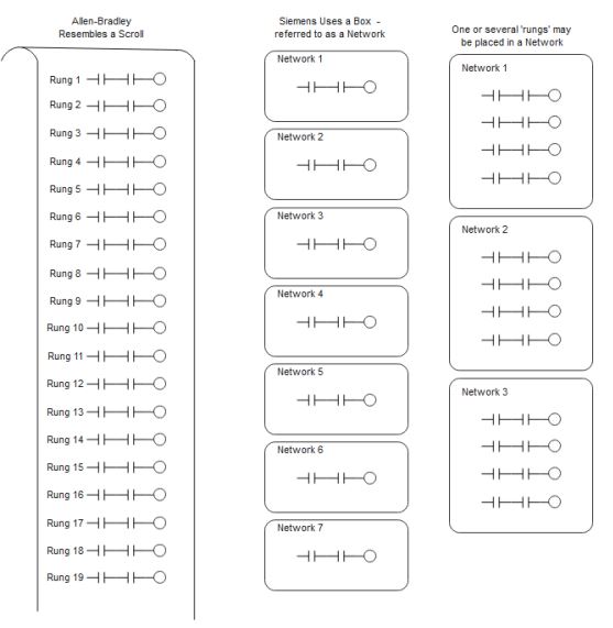
Allen-Bradley and Siemens go about storing programs in a main file that runs continuously in the background of the processor. Allen-Bradley refers to this program as Main while Siemens refers to it as OB1 (Object Block 1). The method of storing logic looks slightly different for the two. At the left is Allen-Bradley’s program format. It resembles a scroll. At right is the Siemens approach. Siemens allows the programmer to use one line or rung of logic per Network or place multiple lines of logic in the same network. An advantage of placing more than one line in the same network is that the logic is not as spread out and can be more easily read.
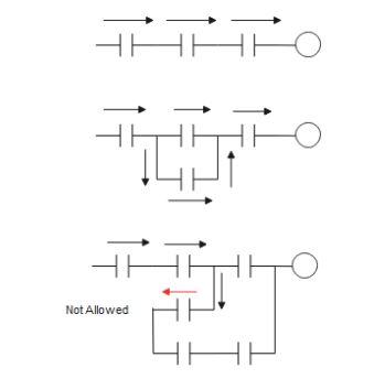
The following shows the path logic is solved by both manufacturers’ PLC. The logic solves left to right, up to down and down to up. Never does the logic flow right to left. There may be a circuit that, if copied as is, would require right to left logic but this logic must be modified to not allow the flow right to left.
Discussion of entry of the logic for both processors is given.
First with Siemens
Organizing the Program in S7
The S7 PLC uses “program containers” called Organization Blocks to separate programs into areas of execution.
OBs are numbered and divided into different classes based on function. The quantity of OBs of a particular class vary by CPU model. OBs are added by the application programmer as desired. OB1 contains the main application program for the PLC. Other OBs can be thought of as interrupt handlers or subroutines (function blocks).
What Are Organization Blocks?
Organization Blocks (OBs) are the interface between the operating system of the CPU and the user program. OBs are used to execute specific program sections:
- At the startup of the CPU
- In a cyclic or clocked execution
- Whenever errors occur
- Whenever hardware interrupts occur
During a warm restart, the first step carried out by the operating system is to delete the non- retentive bit memories, timers, counters, interrupt stack, and block stack; to reset all stored hardware interrupts and diagnostic interrupts; to write the status of the outputs to the PIQ table (Process Image of Outputs); and to start the scan cycle monitoring time. In the second step, the operating system writes the values from the process-image output table into the output modules. In the third step, it then reads the status of the inputs and writes them to the PII Table (Process Image of Inputs). In the fourth step, it then executes the user program with the respective instruction. The operating system starts the cyclic operation again and continually monitors for interrupts.
Startup
A startup program is carried out before the cyclic program execution after a power recovery or a change of operating mode (through the CPU‘s mode selector or by the PG). OB 100 is available in every PLC model, whereas 101 and 102 are only available in the S7-400. In these blocks you can, for example, preset the communications connections or execute initialization routines.
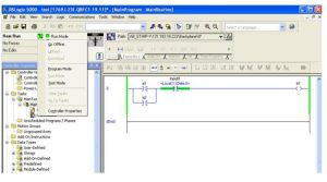
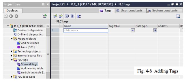
The Program Editor
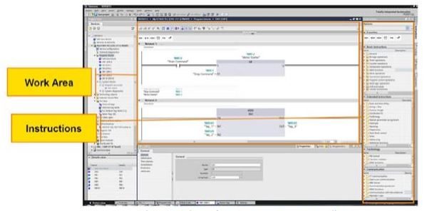
The Editor has the following components:
Instructions
This area shows all instructions available for use in the program. To implement an instruction, select the “rung” (network) you wish to add the instruction to, then “drag and drop” the instruction onto the “rung”.
Work Area
The code section contains the program itself, divided into separate networks (rungs) if required.
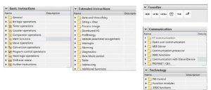
Programming instructions are separated into groups based on functionality.
Basic Instructions – these are the “standard instructions” that can be used with all standard data types. Instructions include Bit Logic Operations, Math functions, Move Operations, and so on.
Extended Instructions – these are instructions that can either be used on complex data types, or that perform specific functions not associated with “traditional” program control functions.
Favorites – you can add frequently used instructions to the Favorites group. Instructions in the Favorites group appear in the upper area of the Program Editor.
Communications – these are instructions used to program communications tasks, such as peer- to- peer PLC communications, open communications over supported networks, and so on.
Technology – these instructions are associated with technology functions supported by the PLC in question. Examples include PID Control.
Addressing Program Elements
As instructions are added, any address the user MUST fill in are shown in a red italic font. The program editor prompts you for the general data format of the instruction as follows:
- ??.? – a bit address
- ??? – an address other than a bit (e.g., byte, word, etc.)
Addresses that can be defined but are not required to be addressed are shown with a black font as an ellipsis (…).
Allowing the mouse pointer to “hover” over an address field will reveal the required data type(s) for the instructions operand. Blocks can be saved without addresses filled in, but the program will not compile until all required addresses are defined.
Programming with Tag Names
You can select configured tags using a pull-down accessible from the instruction. Double clicking will bring an icon into view that can be clicked on to open a list of all tags in the program that have the required data type. You can also start typing and the tags that appear will be filtered based on the text entered to that point. Select the desired tag from the list to assign the tag to the instruction. Autocomplete must be turned on to use this feature.
In many cases, it is necessary to access portions of contiguous data that is “embedded” in a larger tag element. An example would be evaluating or changing a bit address within a word of data.
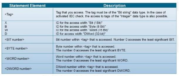
To access a smaller segment of data by a Bit, Byte, Word or Double word, the syntax is as follows:
- BIT <Tag>.x<Bit number>, e.g., “Status Long Word”.X4
- BYTE <Tag>.B<Byte number>, e.g., “Status Long Word”.B2
- WORD <Tag>.W<Word number>, e.g., “Status Long Word”.W0
- DOUBLE WORD <Tag>.D<Double word number>, e.g., “Status Long Word”.D1
Changing an Operand
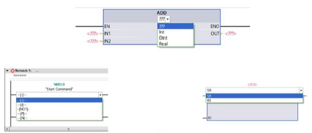
Often it is required to change an operand to a different one. To accomplish this, double click on the instruction, then click on the pull down to select the new operand.
The same feature can be used for many of the math instructions where the data type of the instruction can be changed using the same method.
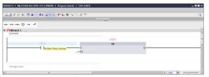
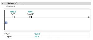
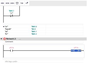
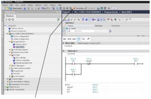
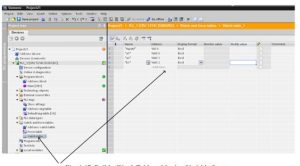
A first contact is chosen and added to the first network, Network 1:
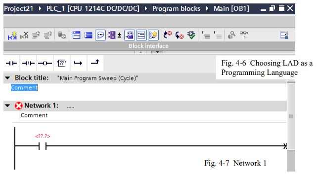
Notice the above the contact. This signals that an address must be selected for this contact, much as a name was required for each contact in a ladder diagram. Move to the tree area PLC tags and choose Show all tags. This area is blank to begin and must be added before the contact above is complete. Bit, byte and word length tags may be created here. Some care must be given to the addressing since tags can be programmed over other tags, a problem that will cause errors later in debugging.
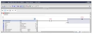
To start, tags will be given generic names such as “a1”, “a2”, etc. This is not a good practice but will be done to start the process of naming variables. Tags should be given meaningful names that give the user an idea as to the meaning behind the contact or other instruction. Below, when the first tag is entered, an address appears of %I0.0. If your tag is to be addressed to the first input %I0.0 then all is well. Usually, this variable needs to be changed. Here it is changed to an M identifier. M bits and bytes are used for internal storage, not for inputs or outputs from the PLC. The first bit of the M table is M0.0. Since this table is addressed in bytes, the succeeding bits are M0.1, M0.2, M0.3, M0.4, M0.5, M0.6, M0.7, M1.0, etc.
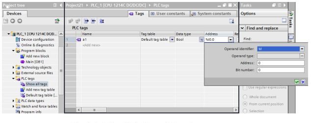
Thus, the first address is entered as M0.0.
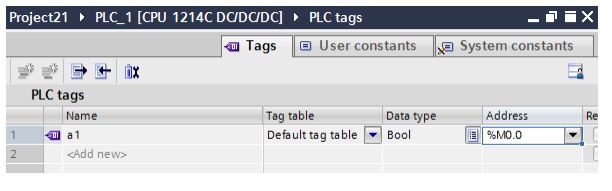
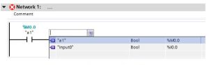
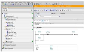
And we proceed back to the ladder diagram for Network 1 and add the tag to the contact:
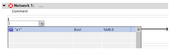
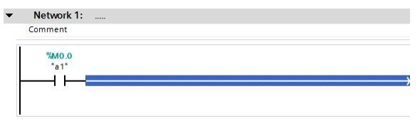
The final result resembles the following:
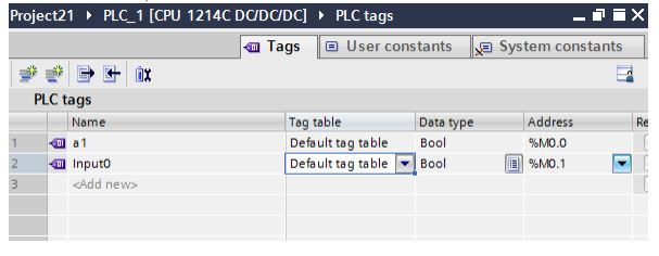
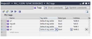
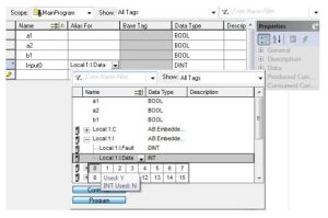
Next, we would like to add an input to the logic. The input is tied to the input point I0.0. In the PLC tag table, we begin with the name “Input0”. We proceed across with default tag table, Bool and then see an address of %M0.1 picked. This must be changed. The tag table will automatically roll to the next available address but we will be using an internal bit for an input but rather an “I” bit, I0.0.
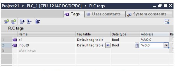
After changing the M address reference to an I address, and entering the correct bit offset, the table appears as follows:
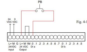
Do not forget that a real device needs to be wired to an input for this input to perform its correct function. Usually the input wired is through a NO (normally open) contact. This may change from time to time but NO is usually chosen.
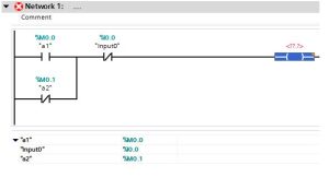
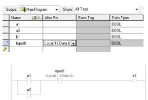
In the Program Block, the contact is added and the tag Input0 chosen.
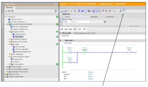
Our program now has a normally closed contact labeled “Input0” address I0.0 in series with a normally open contact labeled “a1” address M0.0. Next, we would like to add a parallel contact to the NO contact “a1”. Start with an arrow from the left ladder.
Add a tag to the tag table ”a2”. Note that we want this address as an M bit so the next available M bit is M0.1.
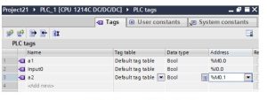
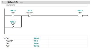
We finish the contact by choosing the normally closed contact and adding the “a2” tag from the tag list:
The up arrow is chosen to tie the circuit right of “a2” to the circuit above. The circuit is now complete except for an output coil.
The output coil is chosen from the instruction list and the tag is added.
The tag is chosen from the internal M bits again, this time M0.2.
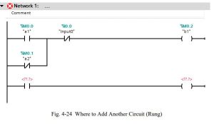
At this time, our circuit is complete. The next rung or circuit is to be programmed in the next available location. The programmer has a choice of moving to the next network, Network2, or continuing in the present network. The program will solve the same either way. Usually, the programmer will continue in the same network for compactness on the screen. More can be seen at the same time when troubleshooting if more rungs are grouped into the same network.
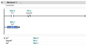
The following shows a second circuit input in the same network as the first. This circuit is not completed but illustrates the ability of the programmer to stack several ideas or circuits into one network.
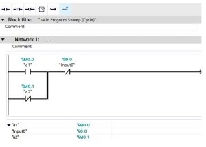
The following shows the same circuit but entered in a second network. Here the ideas are more spread out, usually a less attractive alternative but available as desired.
When defining a Boolean variable, the choice of local or global is to be given. The only time that a variable is to be defined as a Local variable is when the information is only to be passed to a later rung in the same scan but lost after this. The local variable does not return after the end of the scan. Care must be taken to not choose ‘Local’ because it is the default choice. It is not the preferred choice in most cases.
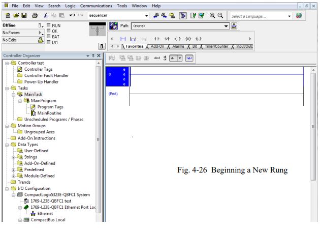
Next, Allen-Bradley
Starting with the project tree, the first program to enter is MainRoutine under MainProgram. This program is equivalent to OB1 in that it is always on and scanning in the background. Execution occurs as often as possible when other programs are not pre-empting the cpu’s time. This program is programmed in Ladder. Subroutines and other programs may be programmed in FBD and STL.
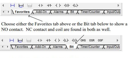
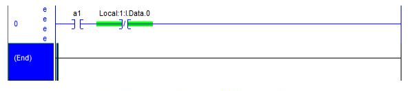
To choose a NO contact, either of the following tabs may be chosen.
Tags are given the same generic names as with the Siemens processor but care must be taken to be meaningful to the process being represented. Names generally are less than 30 characters in length and may have underscore ( _ ). The more well commented, the better in the long run.
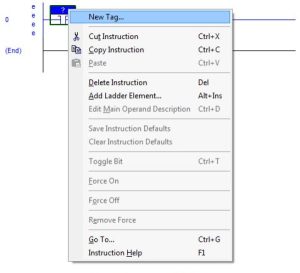
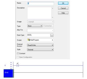
The tag may be entered by right clicking the contact. The new tag will then be entered from the following screens:
The screen below will be entered with Name as a1. A description may be entered if desired. Since the contact was chosen, the Data Type is Bool. Other options are listed but usually left as is.
When the tag name is successfully entered, the contact and tag appear as one unit. It is worth noting that the A-B tag database has no M offsets similar to the Siemens architecture. The variables’ offset is hidden from the user. This is more like a computer language in which the value of a variable’s address may not be known.
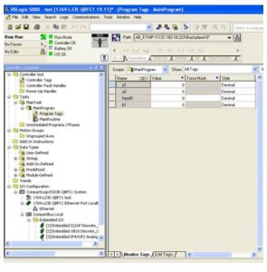
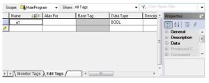
Tags may also be entered from the Program Tags option from the project tree. Here, they are entered in the Edit Tags mode (see tab at bottom of page). This mode must be properly set to enter tags or monitor tags. Use the Monitor Tags mode when online and changing variables to verify the program or enter data to try for a specific result. This tag will be discussed more in the troubleshooting section.
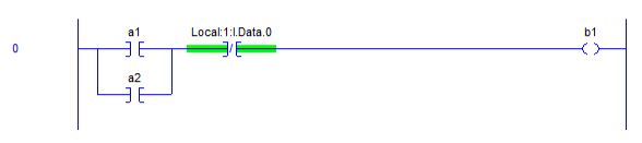
Input and output tags are already defined and may be entered using their address. The addresses for these devices can be found under the controller tab Controller Tags. This table is set for the L23E. Other controllers with stacked cards will vary with the card type and number of each. For our processor, the following I/O list is standard.
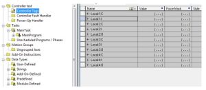
Expand the Input tab to find the specific input point to be used. For input point 0, Local:1:I.Data.0 is used.
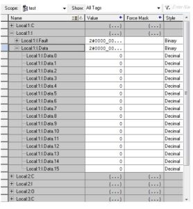
This data address may be copied into the contact directly and used for the address.
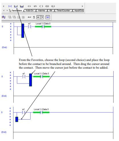
Adding a parallel branch involves the following:
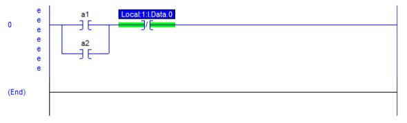
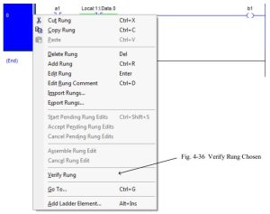
Once the rung has been completed, it is wise to verify the rung for completeness. Right click on the rung at left. The following will appear. Choose Verify Rung and the eee’s should disappear.
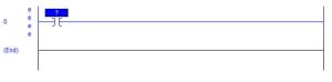
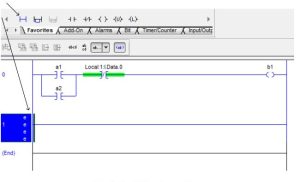
To start a second rung, simply click on the new rung button. The following will appear.
You may alias a tag to another name as shown in the example below. Here Input0 is aliased to
Local:1:I.Data.0.
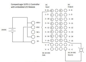
Finally an A-B L16ER processor wired for inputs and outputs:
Troubleshooting the Siemens Processor
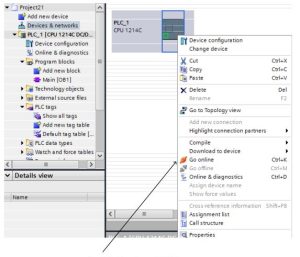
Online mode
In online mode, there is an online connection between your programming device / PC and one or more devices.
An online connection between the programming device/PC and the device is required, for example, for the following tasks:
- Testing user programs
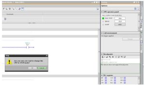
- Displaying and changing the operating mode of the CPU
- Displaying and setting the date and time of day of the CPU
- Displaying module information
- Comparing blocks
Hardware diagnostics
Several changes appear when in the online mode. Among them are the following:
- The title bar of the active window now has an orange background.
- The title bars of inactive windows for the relevant station now have an orange line below them.
- An orange, pulsing bar appears at the right-hand edge of the status bar. If the connection has been established but is functioning incorrectly, an icon for an interrupted connection is displayed instead of the bar. You will find more information on the error in “Diagnostics” in the Inspector window.
- Operating mode symbols or diagnostics symbols for the stations connected online and their underlying objects are shown in the project tree. A comparison of the online and offline status is also made automatically. Differences between online and offline objects are also displayed in the form of symbols.
- The “Diagnostics > Device information” area is brought to the foreground in the Inspector window.
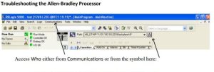
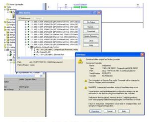
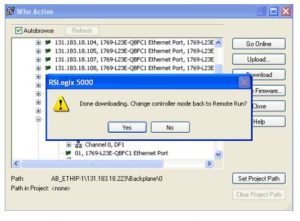
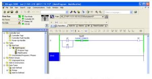
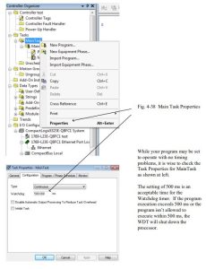
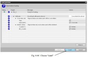
Troubleshooting the Allen-Bradley Processor