
1.4 Math Review
Silly School Songs: The Order of Operations
For the purpose of this course, we will need to learn some basic when dealing with logarithms. We will not, however, delve too deeply into theory and will instead focus on the skills we need.
Exponential Functions[1]
India is the second most populous country in the world with a population of about 1.25 billion people in 2013. The population is growing at a rate of about 1.2% each year[17]. If this rate continues, the population of India will exceed China’s population by the year 2031. When populations grow rapidly, we often say that the growth is “exponential,” meaning that something is growing very rapidly. To a mathematician, however, the term exponential growth has a very specific meaning. In this section, we will take a look at exponential functions, which model this kind of rapid growth.
When exploring linear growth, we observed a constant rate of change—a constant number by which the output increased for each unit increase in input. For example, in the equation  , the slope tells us the output increases by 3 each time the input increases by 1. The scenario in the India population example is different because we have a percent change per unit time (rather than a constant change) in the number of people.
What exactly does it mean to grow exponentially? What does the word double have in common with percent increase? People toss these words around errantly. Are these words used correctly? The words certainly appear frequently in the media.
- Percent change refers to a change based on a percent of the original amount.
- Exponential growth refers to an increase based on a constant multiplicative rate of change over equal increments of time, that is, a percent increase of the original amount over time.
- Exponential decay refers to a decrease based on a constant multiplicative rate of change over equal increments of time, that is, a percent decrease of the original amount over time.
For us to gain a clear understanding of exponential growth, let us contrast exponential growth with linear growth. We will construct two functions. The first function is exponential. We will start with 1 and then we will double the corresponding consecutive outputs. The second function is linear. We will start with an input of 0 and then we will add 2 to the corresponding consecutive outputs. See Table 1.4.1.
|
x
|
y=2x
|
y=2x
|
| Start | 1 | 0 |
| 1 | 2 | 2 |
| 2 | 4 | 4 |
| 3 | 8 | 6 |
| 4 | 16 | 8 |
| 5 | 32 | 10 |
| 6 | 64 | 12 |
| 7 | 128 | 14 |
| 8 | 256 | 16 |
From Table 1.8.1 we can infer that for these two functions, exponential growth dwarfs linear growth.
- Exponential growth refers to the original value from the range increases by the same percentage over equal increments found in the domain.
- Linear growth refers to the original value from the range increases by the same amount over equal increments found in the domain.
Apparently, the difference between “the same percentage” and “the same amount” is quite significant. For exponential growth, over equal increments, the constant multiplicative rate of change resulted in doubling the output whenever the input increased by one. For linear growth, the constant additive rate of change over equal increments resulted in adding 2 to the output whenever the input was increased by one.
The general form of the exponential function is  where
where  is any nonzero number,
  is a positive real number not equal to
  . For our class, will always be greater than one.
Suppose that we have the following exponential equation:
 .
.
If I want to see what the value of  will be when
  , we simply plug
  in for
  . When we do that, we get:
 .
.
As long as we are careful about our order of operations, this is nothing more than a calculator exercise. But what if I want to know what will be equal to when  . How can we get the x down from the exponent? For that, we will need to use the inverse of the exponential…the logarithm.
Let’s try one together…
The elk population of an area is given by the equation below where  is given in number of years:
 .
.
Calculate the number of elk after 5 years. 10 years. 100 years.
Answers: 191; 244; 19,725
College Algebra. Provided by: OpenStax. Located at: https://openstax.org/books/college-algebra/pages/6-3-logarithmic-functions
Logarithms
In order to analyze the magnitude of earthquakes or compare the magnitudes of two different earthquakes, we need to be able to convert between logarithmic and exponential form. For example, suppose the amount of energy released from one earthquake were 500 times greater than the amount of energy released from another. We want to calculate the difference in magnitude. The equation that represents this problem is  , where represents the difference in magnitudes on the Richter Scale. How would we solve for ?
We have not yet learned a method for solving exponential equations. None of the algebraic tools discussed so far is sufficient to solve something like  . We can estimate what needs to be since
  and
and  so the value of has to fall between
  and
and  .
.
The exponential function  is one-to-one, so its inverse,
  is also a function. As is the case with all inverse functions, we simply interchange and and solve for y to find the inverse function. To represent as a function of , we use a logarithmic function of the form

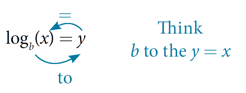
The base logarithm of a number is the exponent by which we must raise to get that number.
We read a logarithmic expression as, “The logarithm with base of is equal to ,” or, simplified, “log base of is .” We can also say, “ raised to the power of is ,” because logs are exponents. For example, the base logarithm of  is
is  , because is the exponent we must apply to to get . Since
 , we can write
  We read this as “log base of is .”
We can express the relationship between logarithmic form and its corresponding exponential form as follows:
Using Your Calculator to Calculate Logarithms
College Algebra. Provided by: OpenStax. Located at: https://openstax.org/books/college-algebra/pages/6-5-logarithmic-properties
Unfortunately, most calculators cannot calculate every single logarithm because there are an infinite number of bases. However, we can use one simple rule to make it possible to calculate the value of any logarithm. Again, we will be focusing on the “how” here and not the “why”.
The most common “base” for the logarithm is base 10 which is also called the common log. On your calculator you should see some “log” button. This is (most likely) to calculate the log base 10. So for instance, if you had the following problem:

we would want to know what we could raise  to in order to get
  . If you enter log(33) (or however you calculator has you enter it — if you are not sure, ask me!), you should get
  which means if you raise to the power you will get
But what if we want to calculate  ?
?
(Most) calculators are not equipped to handle a log of a base other than 10 (and one other that we will talk about soon), but we can use a property to help us.
An important logarithm property is the change-of-base property. This allows us to change the base of the log from one value to another. We will use this to our advantage. The change of base property is as follows:

We will generally use this to convert to the common log (log base 10) so we can run it on a calculator.
When converting to base 10 (the common log), we use the following:

Let us try a few examples!
Let’s try one together…
Evaluate the following logarithms to two decimal places:


Answers: 1.92, 2.28, 4
Solving Exponential Equations[2]
Now let us get back to the problem we were initially looking at. Remember we had explored the following problem:

I had asked what the value of is when is equal to  . So let us plug that in for :

Next, we divide both sides by :

So, now we have

Where do we go next? The logarithm is the inverse operation for the exponential. So for this problem, we need to take the log of base 1.05 of each side. On the left, we get:

On the right, after using change of base, we get

Therefore, 
If we check our work and plug in  for back into our original equation, we get
Let us try a few examples.
Let’s try one together…
when  :
: 
Answer: t=9.269
Let’s try one together…
when  :
: 
Answer: t=66.043
Exponential Growth[3]
We now take a look at what the exponential means. Suppose that we have the equation  This can be rewritten as
  When we add something to , then the quantity is increasing by that amount as a percentage. For example, in our equation we can see that we have
  which means that the quantity is growing by
  or
or  per year (or time period.) A larger value means faster growth and vice versa.
We will see shortly once we start the financial math that this is where the interest rate will come into play.
If the value is less than , then we have decay. For example, if we have  then each year we only have
  or
or  of what we had the previous year. This means that our quantity is decreasing by
  or
or  or
or  each year (or time period.)
We will not use this very often (if ever) in this class.
- Adapted from 12.1 exponential-functions in Personal Finance by lumen learning shared under a CC BY-NC-SA 3.0 license ↵
- New content added to Math of Money edition by J. Z. Klingensmith ↵
- New content added to Math of Money edition by J. Z. Klingensmith[ ↵
