4.2 Elasticity and Revenue
Learning Objectives
By the end of this section, you will be able to:
- Analyze graphs in order to classify elasticity as constant unitary, infinite, or zero
- Describe the price effect and the quantity effect
- Analyze how price elasticities impact revenue and expenditure
In Topic 4.1, we introduced the concept of elasticity and how to calculate it, but we didn’t explain why it is useful. Recall that elasticity measures responsiveness of one variable to changes in another variable. If you owned a coffee shop and wanted to increase your prices, this ‘responsiveness’ is something you need to consider. When you increase prices, you know quantity will fall, but by how much?
Elasticities can be divided into three broad categories: elastic, inelastic, and unitary. An elastic demand is one in which the elasticity is greater than one, indicating a high responsiveness to changes in price. Elasticities that are less than one indicate low responsiveness to price changes and correspond to inelastic demand. Unitary elasticities indicate proportional responsiveness of either demand or supply, as summarized in the following table:
| If . . . | Then . . . | And It Is Called . . . |
|---|---|---|
| [latex]\%\;change\;in\;quantity > \%\;change\;in\;price[/latex] | [latex]\frac{\%\;change\;in\;quantity}{\%\;change\;in\;price)} > 1[/latex] | Elastic |
| [latex]\%\;change\;in\;quantity = \%\;change\;in\;price[/latex] | [latex]\frac{\%\;change\;in\;quantity}{\%\;change\;in\;price)} = 1[/latex] | Unit Elastic |
| [latex]\%\;change\;in\;quantity < \%\;change\;in\;price[/latex] | [latex]\frac{\%\;change\;in\;quantity}{\%\;change\;in\;price)} < 1[/latex] | Inelastic |
| Elastic, Inelastic, and Unitary: Three Cases of Elasticity | ||
If we were to calculate elasticity at every point on a demand curve, we could divide it into these elastic, unit elastic, and inelastic areas, as shown in Figure 4.2a. This means the impact of a price change will depend on where we are producing. Feel free to calculate the elasticity in any of the regions, you will find that it indeed fits the description.
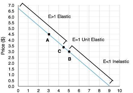
To demonstrate, we have calculated the elasticities at a point in each of the zones:
Point A = [latex]\frac{\Delta Q}{\Delta P}\cdot \frac{P}{Q}=\frac{9}{6.75}\cdot \frac{4.5}{3}=2[/latex] = Elastic
Point B = [latex]\frac{\Delta Q}{\Delta P}\cdot \frac{P}{Q}=\frac{9}{6.75}\cdot \frac{3}{5}=0.8[/latex] = Inelastic
Point C = [latex]\frac{\Delta Q}{\Delta P}\cdot \frac{P}{Q}=\frac{9}{6.75}\cdot \frac{3.375}{4.5}=1[/latex] = Unit Elastic
In reality, the only point we need to find to determine which areas are elastic and inelastic is our point where elasticity is 1, or Point C. This isn’t as hard as it may seem. Since our formula is equal to the inverse of our slope multiplied by a point on the graph, it will only equal 1 when our point is equal to the slope of our graph. For a linear graph, this only occurs at the middle point, which is (4.5, 3.325) in this case.
Why is This Useful?

So far, we have determined how to calculate elasticity at and between different points, but why is this knowledge useful?
Consider a coffee shop owner considering a price hike. The owner has two things to account for when deciding whether to raise the price, one that increases revenue and one that decreases it. Elasticity helps us determine which effect is greater. Referring back to our table:
- When you increase price, you increase revenue on units sold (The Price Effect).
- When you increase price, you sell fewer units (The Quantity Effect).
These two effects work against each-other. To determine which outweighs the other we can look at elasticity:
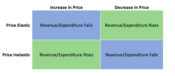
When our point is elastic our [latex]\%\;change\;in\;quantity > \%\;change\;in\;price[/latex] meaning if we increase price, our quantity effect outweighs the price effect, causing a decrease in revenue.
When our point is inelastic our [latex]\%\;change\;in\;quantity < \%\;change\;in\;price[/latex] meaning if we increase price, our price effect outweighs the quantity effect, causing a increase in revenue.
This information is summarized in Figure 4.2b:
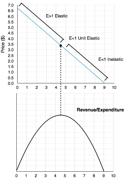
The first thing to note is that revenue is maximized at the point where elasticity is unit elastic. Why? If you are the coffee shop owner, you will notice that there are untapped opportunities when demand is elastic or inelastic.
If elastic: The quantity effect outweighs the price effect, meaning if we decrease prices, the revenue gained from the more units sold will outweigh the revenue lost from the decrease in price.
If inelastic: The price effect outweighs the quantity effect, meaning if we increase prices, the revenue gained from the higher price will outweigh the revenue lost from less units sold.
The effects of price increase and decrease at different points are summarized in Figure 4.2c.
What about Expenditure
You will notice that expenditure is mentioned whenever revenue is. This is because a dollar earned by the coffee shop corresponds to a dollar spent by the consumer. Therefore, if the firm’s revenue is rising, then the consumer’s expenditure is rising as well. You must understand how to answer questions from both sides.
Summary
Elasticity is used to measure the responsiveness of one variable to another. This responsiveness can be labelled as elastic (e > 1), unit elastic (e = 1), and inelastic (e < 1). We can apply this to the demand curve, with unit elastic corresponding to the middle of the demand curve (x-intercept/2 , y-intercept/2). Everything to the left is elastic and everything to the right is inelastic. This information can be used to maximize revenue or expenditure, with the understanding that when elastic, the quantity effect outweighs the price effect, and when inelastic, the price effect outweighs the quantity effect.
Glossary
- Elastic
- when the elasticity is greater than one, indicating that a 1 percent increase in price will result in a more than 1 percent increase in quantity; this indicates a high responsiveness to price.
- Inelastic
- when the elasticity is less than one, indicating that a 1 percent increase in price paid to the firm will result in a less than 1 percent increase in quantity; this indicates a low responsiveness to price.
- Unitary elastic
- when the calculated elasticity is equal to one indicating that a change in the price of the good or service results in a proportional change in the quantity demanded or supplied
Exercises 4.2
Use the demand curve diagram below to answer the following TWO questions.

1. What is the own-price elasticity of demand as price decreases from $8 per unit to $6 per unit? Use the mid-point formula in your calculation.
a) Infinity.
b) 7.0
c) 2.0.
d) 1.75
2. At what point is demand unit-elastic?
a) P = $6, Q = 12.
b) P = $4, Q = 8.
c) P = $2, Q = 12.
d) None of the above.
3. Which of the following statements about the relationship between the price elasticity of demand and revenue is TRUE?
a) If demand is price inelastic, then increasing price will decrease revenue.
b) If demand is price elastic, then decreasing price will increase revenue.
c) If demand is perfectly inelastic, then revenue is the same at any price.
d) Elasticity is constant along a linear demand curve and so too is revenue.
4. Suppose BC Ferries is considering an increase in ferry fares. If doing so results in an increase in revenues raised, which of the following could be the value of the own-price elasticity of demand for ferry rides?
a) 0.5.
b) 1.0.
c) 1.5.
d) All of the above.
5. Use the demand diagram below to answer this question. Note that P × Q equals $900 at every point on this demand curve.
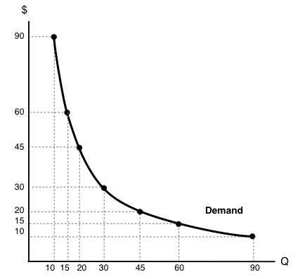
Which of the following statements correctly describes own-price elasticity of demand, for this particular demand curve?
I. Demand is unit elastic at a price of $30, and elastic at all prices greater than $30.
II. Demand is unit elastic at a price of $30, and inelastic at all prices less than $30.
III. Demand is unit elastic for all prices.
a) I and II only.
b) I only.
c) I, II and III.
d) III only.
6. Suppose that, if the price of a good falls from $10 to $8, total expenditure on the good decreases. Which of the following could be the (absolute) value for the own-price elasticity of demand, in the price range considered?
a) 1.6.
b) 2.3.
c) Both a) and b).
d) Neither a) or b).
7. Consider the demand curve drawn below.
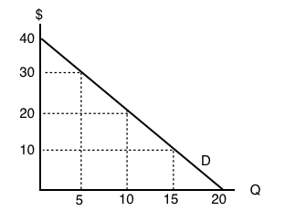
At which of the following prices and quantities is revenue maximized?
a) P = 40; Q = 0.
b) P = 30; Q = 5.
c) P = 20; Q = 10.
d) P = 0; Q = 20.

