3.3 BJT Collector Curves
One of the more useful BJT device plots is the family of collector curves. This is a series of plots of collector current, IC , versus collector-emitter voltage, VCE , at varying levels of base current, IB. To generate these curves we drive the base terminal with a fixed current source establishing IB. A DC power supply is attached from the collector to emitter and then swept from zero volts to some upper value. This establishes VCE . Simultaneously, we track the resulting collector current and plot the result. This results in one trace. The base current is then increased and the DC supply swept again for a second trace. This process is repeated to create a family of curves. An example is shown in Figure 3.3.1.
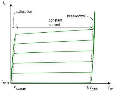
The bottom curve results when IB = 0. Ideally, the corresponding collector current would be 0 but a small leakage current occurs. This is usually referred to as ICEO , meaning the Collector-Emitter current with the base terminal Open (i.e., no base current). The curves above this correspond to increasing levels of base current; each new base current stepping up a fixed amount for each subsequent trace (e.g., 0 μA, 10 μA, 20 μA, 30 μA, etc.).
The most striking thing about this set of curves is that there are three distinct regions or zones of operation. To the extreme left of the curve the current rises rapidly. This is known as the saturation region. The break-over point is fairly small at just a few tenths of a volt. This can be found on a data sheet as VCE(sat) . The saturation region is used in transistor switching applications.
At the extreme right is another region where the collector current rises rapidly. This is called the breakdown region. This is the same effect we saw with individual diodes. We do not wish to operate devices in this region as damage may result. The breakdown voltage is denoted on most data sheets as BVCEO (Collector to Emitter voltage with an Open base). For general purpose devices this will be in the range of 30 to 60 volts or so, but it can be much higher.
In between these two extremes is a region where the collector current is relatively constant, showing only a modest positive slope. This is the constant current region. This is where we want the transistor to operate for applications such as linear amplifiers.
A device called a curve tracer can be used to generate this family of curves in the lab. A very good approximation for β can be determined using these curves. First, we determine the approximate circuit values for IC and VCE , and locate this point on the graph. We then find the nearest plot line to that point. From the intersection of VCE and and this plot line we track back to the vertical axis to find the precise value of IC for that trace. We count the number of traces and multiply by the base current step size to determine the corresponding base current. We then divide the two values and arrive at β.
Example 3.3.1
Assume we have a BJT operating at VCE = 30 V and IC = 4 mA. If the device is placed in a curve tracer and the resulting family of curves appears as in Figure 3.3.2, determine the value of β. Assume the base current is increased 10 μA per trace.
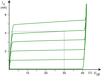
First, find a trace close to the operating point of 30 volts and 4 mA. Draw a vertical line at 30 volts and stop when that line intersects the trace nearest to 4 mA. In this example that’s the second trace from the top. From that intersection point, track back to the vertical axis to determine the precise collector current. That’s roughly 4.2 mA here. To determine the base current count up the number of traces to the selected trace. The selected trace is the fourth one up (do not include the bottom trace where IB is 0). The base current is increased by 10 μA per trace so that leaves us with IB = 40 μA.
![\[\beta=\frac{I_C}{I_B}\]](https://pressbooks.nscc.ca/app/uploads/quicklatex/quicklatex.com-27f95c8dee373efe9b0ad50eb309a67e_l3.png "Rendered by QuickLaTeX.com")
![\[\beta=\frac{4.2mA}{40\mu A}\]](https://pressbooks.nscc.ca/app/uploads/quicklatex/quicklatex.com-57b63124dce15f2a585ba490c7c0eb9d_l3.png "Rendered by QuickLaTeX.com")
![\[\beta=105\]](https://pressbooks.nscc.ca/app/uploads/quicklatex/quicklatex.com-94e2752cee3d86a60e46f66948d68472_l3.png "Rendered by QuickLaTeX.com")
Rise in β and Early Voltage
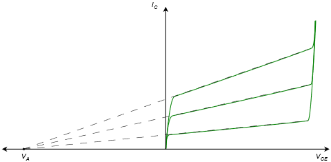
When looking at the collector curves, a good question we might ask is why the collector current rises as VCE increases. This is due to the fact that the increased collector-emitter voltage is responsible for an increase in collector-base voltage (by definition, VCE = VCB + VBE ). VCB is the reverse-bias potential on the collector-base PN junction. As this reverse potential increases, the collector-base depletion region widens. As it widens, it penetrates further into the base layer. Because the base is effectively narrowed, the chances for recombination are reduced, thus reducing base current and effectively increasing β.
If we extend the constant current region traces back into the second quadrant they intersect at a point called the Early Voltage, named after James Early, and denoted as VA . This is illustrated in Figure 3.3.3.