
Excel Practice 5

Prefer to watch and learn? Check out this video tutorial:
Complete the following Practice Activity and submit your completed project.
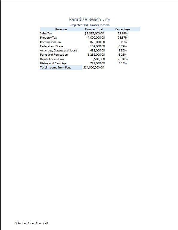
For Excel Practice 5, we will use Excel to manage projected Revenue for Paradise Beach City, where you have just been hired as a Financial Analyst. Key skills in this practice are creating and editing pie charts and What If Analysis.
- On Brightspace in the “Excel Practice 5” sub-module download the Excel starter file provided.
- With the Excel Practice 5 starter file open, Select File, Save As, Browse, and then navigate to your folder on your NSCC OneDrive or other location where you save your files. Name the workbook as Yourlastname_Yourfirstname_Excel_Practice_5.
- To the left of column A, and above row 1, click in the square where the sideways triangle is to select the entire worksheet. AutoFit column width of all cell contents and then click anywhere in the worksheet to deselect it. Ensure you can view all of the cell contents and ### are no longer visible.
- Select the range A1:C1, and merge and center. Apply cell style Title. If the text does not display all the way double-click on the line between the row headings 1 and 2 to Autofit the Row Height.
- Select the range A2:C2, and merge and center. Apply cell style Heading 4.
- Select the range A3:C3 and apply cell style, “Light Blue 20%, Accent1”. Center the headings. Ignore and spelling errors, we will run this later on.
- In cell B12, clear the value in the cell if necessary. Use the AutoSum function to Sum the range B4:B11. You can use any of the methods previously learned to complete the AutoSum function. The formula in cell B12 should look like this =SUM(B4:B11)
- Using the Format Painter, apply the format in cell A3 to A12. To use the Format Painter, select cell A3 so that it is the Active Cell. Click the Format Painter one time to activate it. The Format Painter is located on the Home Tab, in the Clipboard group. With the Format Painter active, click in cell A12.
- In cell C4, type = click cell B4, type / and click cell B12. Make the cell reference B12 absolute in the formula. The formula in cell C4 should look like this = B4/$B$12. This formula will calculate the percentage of third quarter sales tax.
- Select cell C4, and format it as a percentage with two decimal places, and center the percentage. Use the fill handle to copy the formula through cell C11.
- Select the non-adjacent ranges A4:A11 and C4:C11. To select non-adjacent ranges, select the first range, next hold down the CTRL key, and then select the second range letting go of the left mouse button first and then the CTRL key.
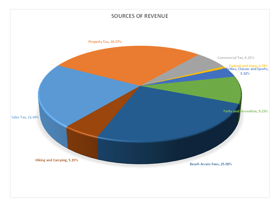
- With the two ranges selected, insert a 3-D Pie Chart. This is located on the Insert Tab, Charts Group, then select the arrow next to Pie Charts and select 3-D Pie Chart.
- Move the chart to a new sheet named Projected Revenue. To create a chart sheet, ensure the chart is selected, on the Chart Tools Design Tab, in the Location Group, select Move Chart. In the Move Chart Dialog Box, select the New Sheet options and type in the name Projected Revenue. Notice how a new sheet is added to the Workbook with the name Projected Revenue.
- Change the chart title to Sources of Revenue. To change the chart title, go to the chart tools design tab, in the chart layouts group, select the arrow next to add chart element and select chart title, above the chart. Left-click on the Chart Title, and type Sources of Revenue pressing Enter when finished.
- With the chart title still selected, change the font size of the title to 36.
- Ensure the entire chart is selected, Using Chart Elements, deselect the Legend check box. Chart Elements is a plus button to the right of the chart.
- Display the Format Data Labels pane. This is on the Chart Tools Design tab, Chart Layout Group, select the arrow next to Add Chart Element, and choose Data Labels and then More Data Labels Options.
- Under Label Options, ensure the only checkboxes checked are Category Name and Percentage. Under Label Position, select, Best Fit. Click the X to close out the Format Data Labels pane.
- Right-click any of the selected data labels, select font, and apply Small Caps and change the font size to 11.
- Select the entire chart area. On the Chart Tools Design Tab, in the Chart Styles Group, select Style 8.
- Double click inside any pie slice to display the Format Data Series pane, click Series Options and ensure Series 1 is selected.
- For Angle of first slice, type 220 and press Enter.
- Under Pie Explosion type 10% and then press Enter. Notice how the slices of pie are separated. Select the Undo button one time, or type 0% for Pie Explosion. Click the X to close the Format Data Series Pane.
- On Sheet1, notice that Beach Access Fees are 8.05%. Click the Projected Revenue tab, and notice how this is represented on the Pie Chart.
- In cell B10 of Sheet1, type 3,500,000 and press Enter. Notice how the percentage automatically changed to 20.63%. Display the chart and notice how this change impacted the Pie Chart.
- Click cell B12 on Sheet1. On the Data tab, in the Forecast Group, click What-If Analysis and click Goal Seek. Goal seeking is the process of finding the correct input value when only the output is known.
- In the Goal Seek dialog box:
- In the Set Cell box, B12 should be displayed.
- In the To value box, type 14000000
- In the By changing cell box, click cell B4.
- Close out of Goal Seek by selecting OK. Double check that cell B12 is set as the Currency number format with two decimal places.
- On the Page Layout Tab, launch the Page Setup Dialog Box and apply the following:
- Center the worksheet Horizontally on the page.
- Insert the File Name in the left footer.
- Rename Sheet1 to Data by double clicking on the “Sheet 1” tab.
- Group All Sheets.
- Press Ctrl + F2 to display the Print Preview. Examine both pages of the workbook. Point out the use of the keyboard shortcut. Show the footer in both sheets.
- In Backstage view, show the advanced properties. Add the following:
- Title: Paradise Beach City Analysis
- Subject: Business Computer Applications, COMP 1050
- Author: Your First and Last Name
- Keywords (Tags): Pie Charts, What-If Analysis, Goal Seek
- If necessary, change the Inventory Sheet to Landscape Orientation.
- Run spelling and grammar check, compare your file to the image below and make all necessary corrections.
- Submit as instructed by your instructor.
Media Attributions
- Practice It Icon © Jessica Parsons is licensed under a CC BY (Attribution) license
