
104 Integrated Rate Laws
[latexpage]
Learning Objectives
By the end of this section, you will be able to:
- Explain the form and function of an integrated rate law
- Perform integrated rate law calculations for zero-, first-, and second-order reactions
- Define half-life and carry out related calculations
- Identify the order of a reaction from concentration/time data
The rate laws discussed thus far relate the rate and the concentrations of reactants. We can also determine a second form of each rate law that relates the concentrations of reactants and time. These are called integrated rate laws. We can use an integrated rate law to determine the amount of reactant or product present after a period of time or to estimate the time required for a reaction to proceed to a certain extent. For example, an integrated rate law is used to determine the length of time a radioactive material must be stored for its radioactivity to decay to a safe level.
Using calculus, the differential rate law for a chemical reaction can be integrated with respect to time to give an equation that relates the amount of reactant or product present in a reaction mixture to the elapsed time of the reaction. This process can either be very straightforward or very complex, depending on the complexity of the differential rate law. For purposes of discussion, we will focus on the resulting integrated rate laws for first-, second-, and zero-order reactions.
First-Order Reactions
Integration of the rate law for a simple first-order reaction (rate = k[A]) results in an equation describing how the reactant concentration varies with time:
where [A]t is the concentration of A at any time t, [A]0 is the initial concentration of A, and k is the first-order rate constant.
For mathematical convenience, this equation may be rearranged to other formats, including direct and indirect proportionalities:
and a format showing a linear dependence of concentration in time:
The Integrated Rate Law for a First-Order ReactionThe rate constant for the first-order decomposition of cyclobutane, C4H8 at 500 °C is 9.2 \(×\) 10−3 s−1:
How long will it take for 80.0% of a sample of C4H8 to decompose?
Solution Since the relative change in reactant concentration is provided, a convenient format for the integrated rate law is:
The initial concentration of C4H8, [A]0, is not provided, but the provision that 80.0% of the sample has decomposed is enough information to solve this problem. Let x be the initial concentration, in which case the concentration after 80.0% decomposition is 20.0% of x or 0.200x. Rearranging the rate law to isolate t and substituting the provided quantities yields:
Check Your Learning Iodine-131 is a radioactive isotope that is used to diagnose and treat some forms of thyroid cancer. Iodine-131 decays to xenon-131 according to the equation:
The decay is first-order with a rate constant of 0.138 d−1. How many days will it take for 90% of the iodine−131 in a 0.500 M solution of this substance to decay to Xe-131?
16.7 days
In the next example exercise, a linear format for the integrated rate law will be convenient:
A plot of ln[A]t versus t for a first-order reaction is a straight line with a slope of −k and a y-intercept of ln[A]0. If a set of rate data are plotted in this fashion but do not result in a straight line, the reaction is not first order in A.
Graphical Determination of Reaction Order and Rate Constant Show that the data in (Figure) can be represented by a first-order rate law by graphing ln[H2O2] versus time. Determine the rate constant for the decomposition of H2O2 from these data.
Solution The data from (Figure) are tabulated below, and a plot of ln[H2O2] is shown in (Figure).
| Trial | Time (h) | [H2O2] (M) | ln[H2O2] |
|---|---|---|---|
| 1 | 0.00 | 1.000 | 0.000 |
| 2 | 6.00 | 0.500 | −0.693 |
| 3 | 12.00 | 0.250 | −1.386 |
| 4 | 18.00 | 0.125 | −2.079 |
| 5 | 24.00 | 0.0625 | −2.772 |
![A graph is shown with the label “Time ( h )” on the x-axis and “l n [ H subscript 2 O subscript 2 ]” on the y-axis. The x-axis shows markings at 6, 12, 18, and 24 hours. The vertical axis shows markings at negative 3, negative 2, negative 1, and 0. A decreasing linear trend line is drawn through five points represented at the coordinates (0, 0), (6, negative 0.693), (12, negative 1.386), (18, negative 2.079), and (24, negative 2.772).](https://pressbooks.nscc.ca/app/uploads/sites/58/2019/07/CNX_Chem_12_04_FrstOKin.jpg)
The plot of ln[H2O2] versus time is linear, indicating that the reaction may be described by a first-order rate law.
According to the linear format of the first-order integrated rate law, the rate constant is given by the negative of this plot’s slope.
The slope of this line may be derived from two values of ln[H2O2] at different values of t (one near each end of the line is preferable). For example, the value of ln[H2O2] when t is 0.00 h is 0.000; the value when t = 24.00 h is −2.772
Check Your Learning Graph the following data to determine whether the reaction \(A\phantom{\rule{0.2em}{0ex}}⟶\phantom{\rule{0.2em}{0ex}}B+C\) is first order.
| Trial | Time (s) | [A] |
|---|---|---|
| 1 | 4.0 | 0.220 |
| 2 | 8.0 | 0.144 |
| 3 | 12.0 | 0.110 |
| 4 | 16.0 | 0.088 |
| 5 | 20.0 | 0.074 |
The plot of ln[A]t vs. t is not linear, indicating the reaction is not first order:
![A graph, labeled above as “l n [ A ] vs. Time” is shown. The x-axis is labeled, “Time ( s )” and the y-axis is labeled, “l n [ A ].” The x-axis shows markings at 5, 10, 15, 20, and 25 hours. The y-axis shows markings at negative 3, negative 2, negative 1, and 0. A slight curve is drawn connecting five points at coordinates of approximately (4, negative 1.5), (8, negative 2), (12, negative 2.2), (16, negative 2.4), and (20, negative 2.6).](https://pressbooks.nscc.ca/app/uploads/sites/58/2020/06/CNX_Chem_12_04_CYL1_img.jpg)
Second-Order Reactions
The equations that relate the concentrations of reactants and the rate constant of second-order reactions can be fairly complicated. To illustrate the point with minimal complexity, only the simplest second-order reactions will be described here, namely, those whose rates depend on the concentration of just one reactant. For these types of reactions, the differential rate law is written as:
For these second-order reactions, the integrated rate law is:
where the terms in the equation have their usual meanings as defined earlier.
The Integrated Rate Law for a Second-Order Reaction The reaction of butadiene gas (C4H6) to yield C8H12 gas is described by the equation:
This “dimerization” reaction is second order with a rate constant equal to 5.76 \(×\) 10−2 L mol−1 min−1 under certain conditions. If the initial concentration of butadiene is 0.200 M, what is the concentration after 10.0 min?
Solution For a second-order reaction, the integrated rate law is written
We know three variables in this equation: [A]0 = 0.200 mol/L, k = 5.76 \(×\) 10−2 L/mol/min, and t = 10.0 min. Therefore, we can solve for [A], the fourth variable:
Therefore 0.179 mol/L of butadiene remain at the end of 10.0 min, compared to the 0.200 mol/L that was originally present.
Check Your Learning If the initial concentration of butadiene is 0.0200 M, what is the concentration remaining after 20.0 min?
0.0195 mol/L
The integrated rate law for second-order reactions has the form of the equation of a straight line:
A plot of \(\frac{1}{\left[A{\right]}_{t}}\) versus t for a second-order reaction is a straight line with a slope of k and a y-intercept of \(\frac{1}{{\left[A\right]}_{0}}.\) If the plot is not a straight line, then the reaction is not second order.
Graphical Determination of Reaction Order and Rate Constant The data below are for the same reaction described in (Figure). Prepare and compare two appropriate data plots to identify the reaction as being either first or second order. After identifying the reaction order, estimate a value for the rate constant.
Solution
| Trial | Time (s) | [C4H6] (M) |
|---|---|---|
| 1 | 0 | 1.00 \(×\) 10−2 |
| 2 | 1600 | 5.04 \(×\) 10−3 |
| 3 | 3200 | 3.37 \(×\) 10−3 |
| 4 | 4800 | 2.53 \(×\) 10−3 |
| 5 | 6200 | 2.08 \(×\) 10−3 |
In order to distinguish a first-order reaction from a second-order reaction, prepare a plot of ln[C4H6]t versus t and compare it to a plot of \(\frac{\text{1}}{\left[{\text{C}}_{4}{\text{H}}_{6}{\right]}_{t}}\) versus t. The values needed for these plots follow.
| Time (s) | \(\frac{1}{\left[{\text{C}}_{4}{\text{H}}_{6}\right]}\phantom{\rule{0.4em}{0ex}}\left({M}^{-1}\right)\) | ln[C4H6] |
|---|---|---|
| 0 | 100 | −4.605 |
| 1600 | 198 | −5.289 |
| 3200 | 296 | −5.692 |
| 4800 | 395 | −5.978 |
| 6200 | 481 | −6.175 |
The plots are shown in (Figure), which clearly shows the plot of ln[C4H6]t versus t is not linear, therefore the reaction is not first order. The plot of \(\frac{1}{\left[{\text{C}}_{4}{\text{H}}_{6}{\right]}_{t}}\) versus t is linear, indicating that the reaction is second order.
![Two graphs are shown, each with the label “Time ( s )” on the x-axis. The graph on the left is labeled, “l n [ C subscript 4 H subscript 6 ],” on the y-axis. The graph on the right is labeled “1 divided by [ C subscript 4 H subscript 6 ],” on the y-axis. The x-axes for both graphs show markings at 3000 and 6000. The y-axis for the graph on the left shows markings at negative 6, negative 5, and negative 4. A decreasing slightly concave up curve is drawn through five points at coordinates that are (0, negative 4.605), (1600, negative 5.289), (3200, negative 5.692), (4800, negative 5.978), and (6200, negative 6.175). The y-axis for the graph on the right shows markings at 100, 300, and 500. An approximately linear increasing curve is drawn through five points at coordinates that are (0, 100), (1600, 198), (3200, 296), and (4800, 395), and (6200, 481).](https://pressbooks.nscc.ca/app/uploads/sites/58/2020/06/CNX_Chem_12_04_2OrdKin.jpg)
According to the second-order integrated rate law, the rate constant is equal to the slope of the \(\frac{1}{\left[A{\right]}_{t}}\) versus t plot. Using the data for t = 0 s and t = 6200 s, the rate constant is estimated as follows:
Check Your Learning Do the following data fit a second-order rate law?
| Trial | Time (s) | [A] (M) |
|---|---|---|
| 1 | 5 | 0.952 |
| 2 | 10 | 0.625 |
| 3 | 15 | 0.465 |
| 4 | 20 | 0.370 |
| 5 | 25 | 0.308 |
| 6 | 35 | 0.230 |
Yes. The plot of \(\frac{1}{\left[A{\right]}_{t}}\) vs. t is linear:
![A graph, with the title “1 divided by [ A ] vs. Time” is shown, with the label, “Time ( s ),” on the x-axis. The label “1 divided by [ A ]” appears left of the y-axis. The x-axis shows markings beginning at zero and continuing at intervals of 10 up to and including 40. The y-axis on the left shows markings beginning at 0 and increasing by intervals of 1 up to and including 5. A line with an increasing trend is drawn through six points at approximately (4, 1), (10, 1.5), (15, 2.2), (20, 2.8), (26, 3.4), and (36, 4.4).](https://pressbooks.nscc.ca/app/uploads/sites/58/2020/06/CNX_Chem_12_04_CYL2_img.jpg)
Zero-Order Reactions
For zero-order reactions, the differential rate law is:
A zero-order reaction thus exhibits a constant reaction rate, regardless of the concentration of its reactant(s). This may seem counterintuitive, since the reaction rate certainly can’t be finite when the reactant concentration is zero. For purposes of this introductory text, it will suffice to note that zero-order kinetics are observed for some reactions only under certain specific conditions. These same reactions exhibit different kinetic behaviors when the specific conditions aren’t met, and for this reason the more prudent term pseudo-zero-order is sometimes used.
The integrated rate law for a zero-order reaction is a linear function:
A plot of [A] versus t for a zero-order reaction is a straight line with a slope of −k and a y-intercept of [A]0. (Figure) shows a plot of [NH3] versus t for the thermal decomposition of ammonia at the surface of two different heated solids. The decomposition reaction exhibits first-order behavior at a quartz (SiO2) surface, as suggested by the exponentially decaying plot of concentration versus time. On a tungsten surface, however, the plot is linear, indicating zero-order kinetics.
Graphical Determination of Zero-Order Rate Constant Use the data plot in (Figure) to graphically estimate the zero-order rate constant for ammonia decomposition at a tungsten surface.
Solution The integrated rate law for zero-order kinetics describes a linear plot of reactant concentration, [A]t, versus time, t, with a slope equal to the negative of the rate constant, −k. Following the mathematical approach of previous examples, the slope of the linear data plot (for decomposition on W) is estimated from the graph. Using the ammonia concentrations at t = 0 and t = 1000 s:
Check Your Learning The zero-order plot in (Figure) shows an initial ammonia concentration of 0.0028 mol L−1 decreasing linearly with time for 1000 s. Assuming no change in this zero-order behavior, at what time (min) will the concentration reach 0.0001 mol L−1?
35 min
![A graph is shown with the label, “Time ( s ),” on the x-axis and, “[ N H subscript 3 ] M,” on the y-axis. The x-axis shows a single value of 1000 marked near the right end of the axis. The vertical axis shows markings at 1.0 times 10 superscript negative 3, 2.0 times 10 superscript negative 3, and 3.0 times 10 superscript negative 3. A decreasing linear trend line is drawn through six points at the approximate coordinates: (0, 2.8 times 10 superscript negative 3), (200, 2.6 times 10 superscript negative 3), (400, 2.3 times 10 superscript negative 3), (600, 2.0 times 10 superscript negative 3), (800, 1.8 times 10 superscript negative 3), and (1000, 1.6 times 10 superscript negative 3). This line is labeled “Decomposition on W.” A decreasing slightly concave up curve is similarly drawn through eight points at the approximate coordinates: (0, 2.8 times 10 superscript negative 3), (100, 2.5 times 10 superscript negative 3), (200, 2.1 times 10 superscript negative 3), (300, 1.9 times 10 superscript negative 3), (400, 1.6 times 10 superscript negative 3), (500, 1.4 times 10 superscript negative 3), and (750, 1.1 times 10 superscript negative 3), ending at about (1000, 0.7 times 10 superscript negative 3). This curve is labeled “Decomposition on S i O subscript 2.”](https://pressbooks.nscc.ca/app/uploads/sites/58/2020/06/CNX_Chem_12_04_AmDecomK.jpg)
The Half-Life of a Reaction
The half-life of a reaction (t1/2) is the time required for one-half of a given amount of reactant to be consumed. In each succeeding half-life, half of the remaining concentration of the reactant is consumed. Using the decomposition of hydrogen peroxide ((Figure)) as an example, we find that during the first half-life (from 0.00 hours to 6.00 hours), the concentration of H2O2 decreases from 1.000 M to 0.500 M. During the second half-life (from 6.00 hours to 12.00 hours), it decreases from 0.500 M to 0.250 M; during the third half-life, it decreases from 0.250 M to 0.125 M. The concentration of H2O2 decreases by half during each successive period of 6.00 hours. The decomposition of hydrogen peroxide is a first-order reaction, and, as can be shown, the half-life of a first-order reaction is independent of the concentration of the reactant. However, half-lives of reactions with other orders depend on the concentrations of the reactants.
First-Order Reactions
An equation relating the half-life of a first-order reaction to its rate constant may be derived from the integrated rate law as follows:
Invoking the definition of half-life, symbolized \({t}_{1\text{/}2},\) requires that the concentration of A at this point is one-half its initial concentration: \(t={t}_{1\text{/}2},\) \(\left[A{\right]}_{t}=\phantom{\rule{0.1em}{0ex}}\frac{1}{2}{\left[A\right]}_{0}.\)
Substituting these terms into the rearranged integrated rate law and simplifying yields the equation for half-life:
This equation describes an expected inverse relation between the half-life of the reaction and its rate constant, k. Faster reactions exhibit larger rate constants and correspondingly shorter half-lives. Slower reactions exhibit smaller rate constants and longer half-lives.
Calculation of a First-order Rate Constant using Half-Life Calculate the rate constant for the first-order decomposition of hydrogen peroxide in water at 40 °C, using the data given in (Figure).
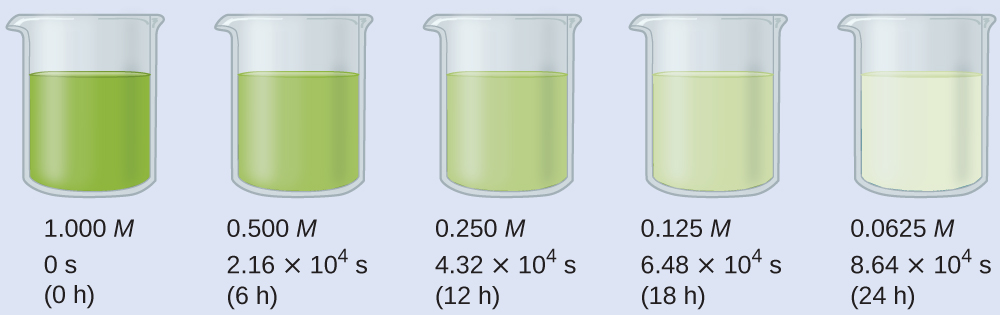
Solution Inspecting the concentration/time data in (Figure) shows the half-life for the decomposition of H2O2 is 2.16 \(×\) 104 s:
Check Your Learning The first-order radioactive decay of iodine-131 exhibits a rate constant of 0.138 d−1. What is the half-life for this decay?
5.02 d.
Second-Order Reactions
Following the same approach as used for first-order reactions, an equation relating the half-life of a second-order reaction to its rate constant and initial concentration may be derived from its integrated rate law:
or
Restrict t to t1/2
define [A]t as one-half [A]0
and then substitute into the integrated rate law and simplify:
For a second-order reaction, \({t}_{1\text{/}2}\) is inversely proportional to the concentration of the reactant, and the half-life increases as the reaction proceeds because the concentration of reactant decreases. Unlike with first-order reactions, the rate constant of a second-order reaction cannot be calculated directly from the half-life unless the initial concentration is known.
Zero-Order Reactions
As for other reaction orders, an equation for zero-order half-life may be derived from the integrated rate law:
Restricting the time and concentrations to those defined by half-life: \(t={t}_{1\text{/}2}\) and \(\left[A\right]=\phantom{\rule{0.1em}{0ex}}\frac{{\left[A\right]}_{0}}{2}.\) Substituting these terms into the zero-order integrated rate law yields:
As for all reaction orders, the half-life for a zero-order reaction is inversely proportional to its rate constant. However, the half-life of a zero-order reaction increases as the initial concentration increases.
Equations for both differential and integrated rate laws and the corresponding half-lives for zero-, first-, and second-order reactions are summarized in (Figure).
| Summary of Rate Laws for Zero-, First-, and Second-Order Reactions | |||
|---|---|---|---|
| Zero-Order | First-Order | Second-Order | |
| rate law | rate = k | rate = k[A] | rate = k[A]2 |
| units of rate constant | M s−1 | s−1 | M−1 s−1 |
| integrated rate law | \(\left[A\right]=\text{−}kt+\left[A{\right]}_{0}\) | \(\text{ln}\left[A\right]=\text{−}kt+\text{ln}\left[A{\right]}_{0}\) | \(\frac{1}{\left[A\right]}\phantom{\rule{0.1em}{0ex}}=kt+\left(\frac{1}{{\left[A\right]}_{0}}\right)\) |
| plot needed for linear fit of rate data | [A] vs. t | ln[A] vs. t | \(\frac{1}{\left[A\right]}\) vs. t |
| relationship between slope of linear plot and rate constant | k = −slope | k = −slope | k = slope |
| half-life | \({t}_{1\text{/}2}=\phantom{\rule{0.1em}{0ex}}\frac{{\left[A\right]}_{0}}{2k}\) | \({t}_{1\text{/}2}=\frac{0.693}{k}\) | \({t}_{1\text{/}2}=\frac{1}{{\left[A\right]}_{0}k}\) |
Half-Life for Zero-Order and Second-Order Reactions What is the half-life (ms) for the butadiene dimerization reaction described in (Figure)?
Solution The reaction in question is second order, is initiated with a 0.200 mol L−1 reactant solution, and exhibits a rate constant of 0.0576 L mol−1 min−1. Substituting these quantities into the second-order half-life equation:
Check Your Learning What is the half-life (min) for the thermal decomposition of ammonia on tungsten (see (Figure))?
18 min
Key Concepts and Summary
Integrated rate laws are mathematically derived from differential rate laws, and they describe the time dependence of reactant and product concentrations.
The half-life of a reaction is the time required to decrease the amount of a given reactant by one-half. A reaction’s half-life varies with rate constant and, for some reaction orders, reactant concentration. The half-life of a zero-order reaction decreases as the initial concentration of the reactant in the reaction decreases. The half-life of a first-order reaction is independent of concentration, and the half-life of a second-order reaction decreases as the concentration increases.
Key Equations
- integrated rate law for zero-order reactions: \(\left[A{\right]}_{t}=\text{−}kt+{\left[A\right]}_{0},\)
- half-life for a ___-order reaction \({t}_{1\text{/}2}=\phantom{\rule{0.1em}{0ex}}\frac{{\left[A\right]}_{0}}{2k}\)
- integrated rate law for first-order reactions: \(\text{ln}\left[A{\right]}_{t}=\text{−}kt+\text{ln}{\left[A\right]}_{0},\)
- half-life for a ___-order reaction \({t}_{1\text{/}2}=\phantom{\rule{0.1em}{0ex}}\frac{0.693}{k}\)
- integrated rate law for second-order reactions: \(\frac{1}{\left[A{\right]}_{t}}\phantom{\rule{0.1em}{0ex}}=kt+\phantom{\rule{0.2em}{0ex}}\frac{1}{{\left[A\right]}_{0}},\)
- half-life for a ___-order reaction \({t}_{1\text{/}2}=\phantom{\rule{0.1em}{0ex}}\frac{1}{{\left[A\right]}_{0}k}\)
Chemistry End of Chapter Exercises
Describe how graphical methods can be used to determine the order of a reaction and its rate constant from a series of data that includes the concentration of A at varying times.
Use the data provided to graphically determine the order and rate constant of the following reaction: \({\text{SO}}_{2}{\text{Cl}}_{2}\phantom{\rule{0.2em}{0ex}}⟶\phantom{\rule{0.2em}{0ex}}{\phantom{\rule{0.2em}{0ex}}\text{SO}}_{2}+{\text{Cl}}_{2}\)
| Time (s) | 0 | 5.00 \(×\) 103 | 1.00 \(×\) 104 | 1.50 \(×\) 104 |
| [SO2Cl2] (M) | 0.100 | 0.0896 | 0.0802 | 0.0719 |
| Time (s) | 2.50 \(×\) 104 | 3.00 \(×\) 104 | 4.00 \(×\) 104 | |
| [SO2Cl2] (M) | 0.0577 | 0.0517 | 0.0415 |
Plotting a graph of ln[SO2Cl2] versus t reveals a linear trend; therefore we know this is a first-order reaction:
![A graph is shown with the label “Time ( s )” on the x-axis and “l n [ S O subscript 2 C l subscript 2 ] M” on the y-axis. The x-axis begins at 0 and extends to 4.00 times 10 superscript 4 with markings every 1.00 times 10 superscript 4. The y-axis shows markings extending from negative 3.5 to negative 2.5. A decreasing linear trend line is drawn through seven points at the approximate coordinates: (0, negative 2.3), (0.5 times 10 superscript 4, negative 2.4), (1.0 times 10 superscript 4, negative 2.5), (1.5 times 10 superscript 4, negative 2.6), (2.0 times 10 superscript 4, negative 2.9), (2.5 times 10 superscript 4, negative 3.0), and (3.0 times 10 superscript 4, negative 3.2).](https://pressbooks.nscc.ca/app/uploads/sites/58/2020/06/CNX_Chem_12_04_Exercise02_img_new.jpg)
k = −2.20 \(×\) 105 s−1
Pure ozone decomposes slowly to oxygen, \({\text{2O}}_{3}\left(g\right)\phantom{\rule{0.2em}{0ex}}⟶\phantom{\rule{0.2em}{0ex}}{\text{3O}}_{2}\left(g\right).\) Use the data provided in a graphical method and determine the order and rate constant of the reaction.
| Time (h) | 0 | 2.0 \(×\) 103 | 7.6 \(×\) 103 | 1.00 \(×\) 104 |
| [O3] (M) | 1.00 \(×\) 10−5 | 4.98 \(×\) 10−6 | 2.07 \(×\) 10−6 | 1.66 \(×\) 10−6 |
| Time (h) | 1.23 \(×\) 104 | 1.43 \(×\) 104 | 1.70 \(×\) 104 | |
| [O3] (M) | 1.39 \(×\) 10−6 | 1.22 \(×\) 10−6 | 1.05 \(×\) 10−6 |
![A graph is shown with the label, “t ( h ,)” on the x-axis and, “1 divided by [ O subscript 3 ] M,” on the y-axis. The x-axis shows markings at 0, 2 times 10 superscript 3, 6 times 10 superscript 3, 10 time 10 superscript 3, 14 times 10 superscript 3, and 18 times 10 superscript 3. The y-axis shows markings beginning at 0, increasing by 1 up to and including 9. An increasing linear trend line is drawn through seven points at the coordinates: (0, 1.00), (2.0 times 10 superscript 3, 2.01), (7.6 times 10 superscript 3, 4.83), (1.00 times 10 superscript 4, 6.02), (1.23 times 10 superscript 4 , 6.02), (1.43 times 10 superscript 4, 8.20) and (1.70 times 10 superscript 4, 9.52). A horizontal line segment is drawn through the first point and a vertical line segment is similarly drawn through the last point to make a right triangle on the graph. The horizontal leg of the triangle is labeled “ capital delta t.” The vertical leg is labeled “capital delta 1 divided by [ O subscript 3 ].”](https://pressbooks.nscc.ca/app/uploads/sites/58/2020/06/CNX_Chem_12_04_Exercise04_img_new.jpg)
The plot is nicely linear, so the reaction is second order. k = 50.1 L mol−1 h−1
From the given data, use a graphical method to determine the order and rate constant of the following reaction:
\(2X\phantom{\rule{0.2em}{0ex}}⟶\phantom{\rule{0.2em}{0ex}}Y+Z\)
| Time (s) | 5.0 | 10.0 | 15.0 | 20.0 | 25.0 | 30.0 | 35.0 | 40.0 |
| [X] (M) | 0.0990 | 0.0497 | 0.0332 | 0.0249 | 0.0200 | 0.0166 | 0.0143 | 0.0125 |
What is the half-life for the first-order decay of phosphorus-32? \(\left({}_{15}^{32}\text{P}\phantom{\rule{0.2em}{0ex}}⟶\phantom{\rule{0.2em}{0ex}}{}_{16}^{32}\text{S}+{\text{e}}^{-}\right)\) The rate constant for the decay is 4.85 \(×\) 10−2 day−1.
14.3 d
What is the half-life for the first-order decay of carbon-14? \(\left({}_{\phantom{\rule{0.5em}{0ex}}6}^{14}\text{C}⟶{}_{\phantom{\rule{0.5em}{0ex}}7}^{14}\text{N}+{\text{e}}^{-}\right)\) The rate constant for the decay is 1.21 \(×\) 10−4 year−1.
What is the half-life for the decomposition of NOCl when the concentration of NOCl is 0.15 M? The rate constant for this second-order reaction is 8.0 \(×\) 10−8 L mol−1 s−1.
8.3 \(×\) 107 s
What is the half-life for the decomposition of O3 when the concentration of O3 is 2.35 \(×\) 10−6M? The rate constant for this second-order reaction is 50.4 L mol−1 h−1.
The reaction of compound A to give compounds C and D was found to be second-order in A. The rate constant for the reaction was determined to be 2.42 L mol−1 s−1. If the initial concentration is 0.500 mol/L, what is the value of t1/2?
0.826 s
The half-life of a reaction of compound A to give compounds D and E is 8.50 min when the initial concentration of A is 0.150 M. How long will it take for the concentration to drop to 0.0300 M if the reaction is (a) first order with respect to A or (b) second order with respect to A?
Some bacteria are resistant to the antibiotic penicillin because they produce penicillinase, an enzyme with a molecular weight of 3 \(×\) 104 g/mol that converts penicillin into inactive molecules. Although the kinetics of enzyme-catalyzed reactions can be complex, at low concentrations this reaction can be described by a rate law that is first order in the catalyst (penicillinase) and that also involves the concentration of penicillin. From the following data: 1.0 L of a solution containing 0.15 µg (0.15 \(×\) 10−6 g) of penicillinase, determine the order of the reaction with respect to penicillin and the value of the rate constant.
| [Penicillin] (M) | Rate (mol L−1 min−1) |
|---|---|
| 2.0 \(×\) 10−6 | 1.0 \(×\) 10−10 |
| 3.0 \(×\) 10−6 | 1.5 \(×\) 10−10 |
| 4.0 \(×\) 10−6 | 2.0 \(×\) 10−10 |
The reaction is first order. k = 1.0 \(×\) 107 L mol−1 min−1
Both technetium-99 and thallium-201 are used to image heart muscle in patients with suspected heart problems. The half-lives are 6 h and 73 h, respectively. What percent of the radioactivity would remain for each of the isotopes after 2 days (48 h)?
There are two molecules with the formula C3H6. Propene, \({\text{CH}}_{3}\text{CH}={\text{CH}}_{2},\) is the monomer of the polymer polypropylene, which is used for indoor-outdoor carpets. Cyclopropane is used as an anesthetic:
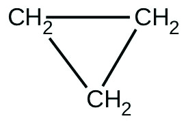
When heated to 499 °C, cyclopropane rearranges (isomerizes) and forms propene with a rate constant of
5.95 \(×\) 10−4 s−1. What is the half-life of this reaction? What fraction of the cyclopropane remains after 0.75 h at 499 °C?
1.67 × 10³ s ; 20% remains
Fluorine-18 is a radioactive isotope that decays by positron emission to form oxygen-18 with a half-life of 109.7 min. (A positron is a particle with the mass of an electron and a single unit of positive charge; the equation is \(\phantom{\rule{0.5em}{0ex}}{}_{9}^{\phantom{\rule{-0.5em}{0ex}}18}\text{F}⟶{}_{18}^{\phantom{\rule{0.5em}{0ex}}8}\text{O}+{}_{+1}^{\phantom{\rule{0.5em}{0ex}}0}\text{e}\right)\) Physicians use 18F to study the brain by injecting a quantity of fluoro-substituted glucose into the blood of a patient. The glucose accumulates in the regions where the brain is active and needs nourishment.
(a) What is the rate constant for the decomposition of fluorine-18?
(b) If a sample of glucose containing radioactive fluorine-18 is injected into the blood, what percent of the radioactivity will remain after 5.59 h?
(c) How long does it take for 99.99% of the 18F to decay?
Suppose that the half-life of steroids taken by an athlete is 42 days. Assuming that the steroids biodegrade by a first-order process, how long would it take for \(\frac{1}{64}\) of the initial dose to remain in the athlete’s body?
252 days
Recently, the skeleton of King Richard III was found under a parking lot in England. If tissue samples from the skeleton contain about 93.79% of the carbon-14 expected in living tissue, what year did King Richard III die? The half-life for carbon-14 is 5730 years.
Nitroglycerine is an extremely sensitive explosive. In a series of carefully controlled experiments, samples of the explosive were heated to 160 °C and their first-order decomposition studied. Determine the average rate constants for each experiment using the following data:
| Initial [C3H5N3O9] (M) | 4.88 | 3.52 | 2.29 | 1.81 | 5.33 | 4.05 | 2.95 | 1.72 |
| t (s) | 300 | 300 | 300 | 300 | 180 | 180 | 180 | 180 |
| % Decomposed | 52.0 | 52.9 | 53.2 | 53.9 | 34.6 | 35.9 | 36.0 | 35.4 |
| [A]0 (M) | k\(×\) 103 (s−1) |
|---|---|
| 4.88 | 2.45 |
| 3.52 | 2.51 |
| 2.29 | 2.53 |
| 1.81 | 2.58 |
| 5.33 | 2.36 |
| 4.05 | 2.47 |
| 2.95 | 2.48 |
| 1.72 | 2.43 |
For the past 10 years, the unsaturated hydrocarbon 1,3-butadiene \(\left({\text{CH}}_{\text{2}}=\text{CH}–\text{CH}={\text{CH}}_{2}\right)\) has ranked 38th among the top 50 industrial chemicals. It is used primarily for the manufacture of synthetic rubber. An isomer exists also as cyclobutene:
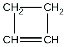
The isomerization of cyclobutene to butadiene is first-order and the rate constant has been measured as 2.0 \(×\) 10−4 s−1 at 150 °C in a 0.53-L flask. Determine the partial pressure of cyclobutene and its concentration after 30.0 minutes if an isomerization reaction is carried out at 150 °C with an initial pressure of 55 torr.
Glossary
- half-life of a reaction (tl/2)
- time required for half of a given amount of reactant to be consumed
- integrated rate law
- equation that relates the concentration of a reactant to elapsed time of reaction
