
11.8 Noise
Generally speaking, noise refers to undesired output signals. The background hiss found on audio tape is a good example of noise. If noise levels get too high, the desired signals are lost. We will narrow our definition down a bit by only considering noise signals that are created by the op amp circuit. Noise comes from a variety of places. First of all, all resistors have thermal, or Johnson noise. This is due to the random effects that thermal energy produces on the electrons. Thermal noise is also called white noise, because it is equally distributed across the frequency spectrum. Semiconductors exhibit other forms of noise. Shot noise is caused by the fact the charges move as discrete particles (electrons). It is also white. Popcorn noise is dominant at lower frequencies and is caused by manufacturing imperfections. Finally, flicker noise has a 1/𝑓 spectral density. This means that it increases as the frequency drops. It is sometimes referred to as 1/𝑓 noise.
Any op amp circuit exhibits noise from all of these sources. Because we are not designing the op amps, we don’t really need to distinguish the exact sources of the noise, rather, we’d just like to find out how much total noise arrives at the output. This will allow us to determine the signal-to-noise ratio (S/N) of the circuit, or how quiet the amplifier is.
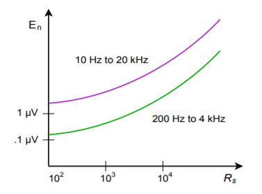
If noise performance for a particular design is not paramount, it can be quickly estimated from manufacturer’s data sheets. Some manufacturers will specify RMS noise voltages for specified signal bandwidths and source impedances. A typical plot is found in Figure 5.8.1 . To use this, simply find the source impedance of your circuit on the horizontal axis, and by using the appropriate signal bandwidth curve, find the noise voltage on the vertical axis. This noise voltage is input-referred. In order to find the output noise voltage, multiply this number by the noise gain of the circuit. The result will not be exact, but it will put you in the ballpark.
A more exact approach involves the use of two op amp parameters, input noise voltage density, 𝑣𝑖𝑛𝑑 , and input noise current density, 𝑖𝑖𝑛𝑑 . Nanovolts per root Hertz are used to specify 𝑣𝑖𝑛𝑑 . Picoamps per root Hertz are used to specify 𝑖𝑖𝑛𝑑 . Refer to the 5534 data sheet for example specifications. (Some manufacturer’s square these values and give units of volts squared per Hertz and amps squared per Hertz. To translate to the more common form, just take the square root of the values given. The data sheet for the 741 is typical of this form). These two parameters take into account noise from all internal sources. As a result, these parameters are frequency dependent. Due to the flicker noise component, the curves tend to be rather flat at higher frequencies and then suddenly start to increase at lower frequencies. The point at which the graphs start to rise is called the noise corner frequency. Generally, the lower this frequency, the better.
In order to find the output noise we will combine the noise from three sources:
- 𝑣𝑖𝑛𝑑
- 𝑖𝑖𝑛𝑑
- The thermal noise of the input and feedback resistors
Before we start, there are a few points to note. First, the strength of the noise is dependent on the noise bandwidth of the circuit. For general-purpose circuits with 20 dB/decade rolloffs, the noise-bandwidth, 𝐵𝑊𝑛𝑜𝑖𝑠𝑒 , is 1.57 times larger than the small-signal bandwidth. It is larger because some noise still exists in the rolloff region. The noise-bandwidth would only equal the small-signal bandwidth if the rolloff rate were infinitely fast. Second, because the noise-bandwidth factor is common to all three sources, instead of calculating its effect three times, we will combine the partial results of the three sources first, and then apply the noise bandwidth effect. This will make the calculation faster, as we have effectively factored out 𝐵𝑊𝑛𝑜𝑖𝑠𝑒 . Each of the three sources will be noise voltage densities, all having units of volts per root Hertz. Because 𝑣𝑖𝑛𝑑 is already in this form, we only need to calculate the thermal and 𝑖𝑖𝑛𝑑 effects before doing the summation. Finally, because noise signals are random, they do not add coherently. In order to find the effective sum we must perform an RMS summation, that is, a square root of the sum of the squares. This will result in the input noise voltage. To find the output noise voltage we will then multiply by 𝐴𝑛𝑜𝑖𝑠𝑒 .
The first thing that must be done is to determine the input noise resistance. 𝑅𝑛𝑜𝑖𝑠𝑒 is the combination of the resistance seen from the inverting input to ground and from the noninverting input to ground. To do this, short the voltage source and ground the output. You will end up with circuit like Figure 5.8.2 . Note that 𝑅𝑖 and 𝑅𝑓 are effectively in parallel. Therefore,
![\[R_{noise} = R_s + R_i || R_f \]](https://pressbooks.nscc.ca/app/uploads/quicklatex/quicklatex.com-fcfded05d2b6c003dfb178671108a855_l3.png "Rendered by QuickLaTeX.com")
(5.8.1)
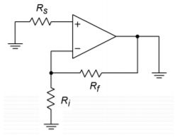
You might note that 𝑅𝑠 is in the same position as 𝑅𝑜𝑓𝑓 for the offset calculations. For absolute minimum noise, the offset compensating resistor is not used. 𝑅𝑛𝑜𝑖𝑠𝑒 is used to find the thermal noise and the contribution of 𝑖𝑖𝑛𝑑 . As always, Ohm’s Law still applies, so as you might expect, 𝑖𝑖𝑛𝑑 𝑅𝑛𝑜𝑖𝑠𝑒 produces a noise voltage density with our desired units of volts per root Hertz. The only source left is the thermal noise.
The general Equation for thermal noise is:
![\[e_{th} =\sqrt{4 K T BW_{noise} R_{noise}} \]](https://pressbooks.nscc.ca/app/uploads/quicklatex/quicklatex.com-2d2311b033f461bec8dc866669e63de4_l3.png "Rendered by QuickLaTeX.com")
(5.8.2)
Where
𝑒𝑡ℎ is the thermal noise.
𝐾 is Boltzmann’s constant, 1.38⋅10−23 Joules/Kelvin degree.
𝑇 is the temperature in Kelvin degrees (Celsius + 273).
𝐵𝑊𝑛𝑜𝑖𝑠𝑒 is the effective noise bandwidth.
𝑅𝑛𝑜𝑖𝑠𝑒 is the equivalent noise resistance.
Because we are interested in finding the noise density, we can pull out the 𝐵𝑊𝑛𝑜𝑖𝑠𝑒 factor. Also, when we perform the RMS summation, this quantity will need to be squared. Instead of taking the square root and then squaring it again, we can just leave it as 𝑒2𝑡ℎ . These two considerations leave us with the mean squared thermal noise voltage density, or
![\[e_{th}^{2} = 4 K T R_{noise} \]](https://pressbooks.nscc.ca/app/uploads/quicklatex/quicklatex.com-fccae091e3d2791efc52d9e53d38d020_l3.png "Rendered by QuickLaTeX.com")
(5.8.3)
Now that we have the components, we may perform the summation.
![\[e_{total} =\sqrt{v_{ind}^{2} +(i_{ind}\times R_{noise})^{2} + e_{th}^{2} } \]](https://pressbooks.nscc.ca/app/uploads/quicklatex/quicklatex.com-25a7dd6e2ca0c96e780726ed514c35b7_l3.png "Rendered by QuickLaTeX.com")
(5.8.4)
The total input noise voltage density is 𝑒𝑡𝑜𝑡𝑎𝑙 . Its units are in volts per root Hertz. At this point we may now include the noise bandwidth effect. In order to find 𝐵𝑊𝑛𝑜𝑖𝑠𝑒 , multiply the small-signal bandwidth by 1.57. If the amplifier is DC coupled, the small-signal bandwidth is equal to 𝑓2 , otherwise it is equal to 𝑓2−𝑓1 . For most applications setting the bandwidth to 𝑓2 is sufficient.
![\[BW_{noise} = 1.57 f_2 \]](https://pressbooks.nscc.ca/app/uploads/quicklatex/quicklatex.com-d1d729e262a88320c5b31d915916cadb_l3.png "Rendered by QuickLaTeX.com")
(5.8.5)
For the final step, 𝑒𝑡𝑜𝑡𝑎𝑙 is multiplied by the square root of 𝐵𝑊𝑛𝑜𝑖𝑠𝑒 . Note that the units for 𝑒𝑡𝑜𝑡𝑎𝑙 are volts per root Hertz. Consequently, we need a root Hertz bandwidth. We are performing a mathematical shortcut here. You could square 𝑒𝑡𝑜𝑡𝑎𝑙 in order to get units of volts squared per Hertz, multiply by 𝐵𝑊𝑛𝑜𝑖𝑠𝑒 , and then take the square root of the result to get back to units of volts, but the first way is quicker. Anyway, we end up with the input referred RMS noise voltage.
![\[e_n = e_{total} \sqrt{BW_{noise}} \]](https://pressbooks.nscc.ca/app/uploads/quicklatex/quicklatex.com-dabe7a5f0a6b7326d90443a85cf7bbd0_l3.png "Rendered by QuickLaTeX.com")
(5.8.6)
Example 5.14
Determine the output noise voltage for the circuit of Figure 5.8.3 . For a nominal output of 1 V RMS, what is the signal-to-noise ratio? Assume T = 300 ∘ K (room temperature).
The 5534 shows the following specs, 𝑣𝑖𝑛𝑑=4𝑛𝑉/𝐻𝑧‾‾‾‾√ , 𝑖𝑖𝑛𝑑=0.6𝑝𝐴/𝐻𝑧‾‾‾‾√ . These values do rise at lower frequencies, but we will ignore this effect for now. Also, 𝑓𝑢𝑛𝑖𝑡𝑦 is 10 MHz.
![\[A_v = 1+ \frac{R_f}{R_i} \]](https://pressbooks.nscc.ca/app/uploads/quicklatex/quicklatex.com-3fead3440157629d6ec728f5898786be_l3.png "Rendered by QuickLaTeX.com")
![\[A_v = 1+ \frac{99 k}{1 k} \]](https://pressbooks.nscc.ca/app/uploads/quicklatex/quicklatex.com-5ad0447dd4dc09e7fe350979d1fc745c_l3.png "Rendered by QuickLaTeX.com")
![\[A_v = 100 \]](https://pressbooks.nscc.ca/app/uploads/quicklatex/quicklatex.com-166a2938648283c348ff526dea108950_l3.png "Rendered by QuickLaTeX.com")
![\[A_{v}^{'} =40 dB \]](https://pressbooks.nscc.ca/app/uploads/quicklatex/quicklatex.com-9bcbf03693b092772193c9fb20b0e14f_l3.png "Rendered by QuickLaTeX.com")
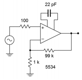
For the noninverting amplifier, 𝐴𝑣=𝐴𝑛𝑜𝑖𝑠𝑒 , so
![\[A_{noise} = 100 = 40 dB \]](https://pressbooks.nscc.ca/app/uploads/quicklatex/quicklatex.com-d2d34ee75cd65899e6bf754d01c1d228_l3.png "Rendered by QuickLaTeX.com")
![\[R_{noise} = R_s + R_f || R_i \]](https://pressbooks.nscc.ca/app/uploads/quicklatex/quicklatex.com-3c068f2fa14ba11ae2343546431081e3_l3.png "Rendered by QuickLaTeX.com")
![\[R_{noise} = 100 + 99 k || 1 k \]](https://pressbooks.nscc.ca/app/uploads/quicklatex/quicklatex.com-f1ecf7e0674901cecc427467e4b5a80a_l3.png "Rendered by QuickLaTeX.com")
![\[R_{noise} = 1090 \Omega \]](https://pressbooks.nscc.ca/app/uploads/quicklatex/quicklatex.com-0e6457d7ca211af8b865c583994c6f84_l3.png "Rendered by QuickLaTeX.com")
![\[e_{th}^{2} = 4\times 1.38\times 10^{-23} \times 300\times 1090 \]](https://pressbooks.nscc.ca/app/uploads/quicklatex/quicklatex.com-e05af972f323d06bf7ad0a26e333ff0d_l3.png "Rendered by QuickLaTeX.com")
![\[e_{th}^{2} = 1.805\times 10^{-17} \text{ Volts squared per Hertz} \]](https://pressbooks.nscc.ca/app/uploads/quicklatex/quicklatex.com-a2f2cbc05c25c48db4f13f5d02048678_l3.png "Rendered by QuickLaTeX.com")
![\[e_{total} = \sqrt{v_{ind}^{2} + (i_{ind} R_{noise})^{2} + e_{th}^{2}} \]](https://pressbooks.nscc.ca/app/uploads/quicklatex/quicklatex.com-fb32a3cab4844a11917bf6ce1435ac73_l3.png "Rendered by QuickLaTeX.com")
![\[e_{total} = \sqrt{(4nV/ \sqrt{Hz})^{2} + (.6 pA/\sqrt{Hz} \times 1090 \Omega)^2 + 1.805\times 10^{−17} V^2/Hz } \]](https://pressbooks.nscc.ca/app/uploads/quicklatex/quicklatex.com-485d33c56984a0112c6dd2822213901e_l3.png "Rendered by QuickLaTeX.com")
![\[e_{total} = \sqrt{1.6\times 10^{-17} + 4.277\times 10^{-19} + 1.805\times 10^{-17} } \]](https://pressbooks.nscc.ca/app/uploads/quicklatex/quicklatex.com-31a3dace9c8e5155e6e3d7904031c309_l3.png "Rendered by QuickLaTeX.com")
![\[e_{total} = 5.87 nV/ \sqrt{Hz} \]](https://pressbooks.nscc.ca/app/uploads/quicklatex/quicklatex.com-ebacf76201e2a90f8e633b202805cf18_l3.png "Rendered by QuickLaTeX.com")
Note that the major noise contributors are 𝑣𝑖𝑛𝑑 and 𝑒𝑡ℎ . Now to find 𝐵𝑊𝑛𝑜𝑖𝑠𝑒 .
![\[f_2 = \frac{f_{unity}}{A_{noise}} \]](https://pressbooks.nscc.ca/app/uploads/quicklatex/quicklatex.com-bc9cf373e611e121da122c2c7cce4043_l3.png "Rendered by QuickLaTeX.com")
![\[f_2 = \frac{10 MHz}{100} \]](https://pressbooks.nscc.ca/app/uploads/quicklatex/quicklatex.com-110dc17a746a20b18447f45992cedbe2_l3.png "Rendered by QuickLaTeX.com")
![\[f_2 = 100 kHz \]](https://pressbooks.nscc.ca/app/uploads/quicklatex/quicklatex.com-2b327a3a84e5b0539fd3cf0fd6a38e92_l3.png "Rendered by QuickLaTeX.com")
![\[BW_{noise} = f_2 1.57 \]](https://pressbooks.nscc.ca/app/uploads/quicklatex/quicklatex.com-039f98a60fc847c4ebf193a197097b54_l3.png "Rendered by QuickLaTeX.com")
![\[BW_{noise} = 100 kHz\times 1.57 \]](https://pressbooks.nscc.ca/app/uploads/quicklatex/quicklatex.com-279095921518e34822db988999bef13d_l3.png "Rendered by QuickLaTeX.com")
![\[BW_{noise} = 157 kHz \]](https://pressbooks.nscc.ca/app/uploads/quicklatex/quicklatex.com-5066a5e4964c4771bfb993b14b54446f_l3.png "Rendered by QuickLaTeX.com")
![\[e_n = 5.87 nV/\sqrt{Hz} \sqrt{157 kHz} \]](https://pressbooks.nscc.ca/app/uploads/quicklatex/quicklatex.com-361a648716c73963540783b2f849daa8_l3.png "Rendered by QuickLaTeX.com")
![\[e_n = 2.33\mu V RMS \]](https://pressbooks.nscc.ca/app/uploads/quicklatex/quicklatex.com-7137cec5c95fd67c104db7e32c9dd882_l3.png "Rendered by QuickLaTeX.com")
To find the output noise, multiply by the noise gain.
![\[e_{n-out} = e_n A_{noise} \]](https://pressbooks.nscc.ca/app/uploads/quicklatex/quicklatex.com-5a9e21f270e068cef52b6666f6a89ccf_l3.png "Rendered by QuickLaTeX.com")
![\[e_{n-out} = 2.33\mu V\times 100 \]](https://pressbooks.nscc.ca/app/uploads/quicklatex/quicklatex.com-517d6e8bb9f07b2f6b8f1726e717a3b2_l3.png "Rendered by QuickLaTeX.com")
![\[e_{n-out} = 233\mu V RMS \]](https://pressbooks.nscc.ca/app/uploads/quicklatex/quicklatex.com-232007e2943bd722fc01c819fa09ad1b_l3.png "Rendered by QuickLaTeX.com")
For a nominal output signal of 1 V RMS, the signal-to-noise ratio is
![\[S/N = \frac{Signal}{Noise} \]](https://pressbooks.nscc.ca/app/uploads/quicklatex/quicklatex.com-5be036229b20e1f3438a53f5f04da71f_l3.png "Rendered by QuickLaTeX.com")
![\[S/N = \frac{1 V}{233\mu V} \]](https://pressbooks.nscc.ca/app/uploads/quicklatex/quicklatex.com-da5d53e7e3511092a1cb8b4eefcde6be_l3.png "Rendered by QuickLaTeX.com")
![\[S/N = 4290 \]](https://pressbooks.nscc.ca/app/uploads/quicklatex/quicklatex.com-4fff83bfc3b9d60ffda075322fece30a_l3.png "Rendered by QuickLaTeX.com")
Normally S/N is given in dB
![\[S/N^{'} = 20 \log_{10} S/N \]](https://pressbooks.nscc.ca/app/uploads/quicklatex/quicklatex.com-4fd8cba0e62e1401f45c9cf9de7730c4_l3.png "Rendered by QuickLaTeX.com")
![\[S/N^{'} = 20 \log_{10} 4290 \]](https://pressbooks.nscc.ca/app/uploads/quicklatex/quicklatex.com-fde75bdad344159a0364c6ff0d071ad5_l3.png "Rendered by QuickLaTeX.com")
![\[S/N^{'} = 72.6 dB \]](https://pressbooks.nscc.ca/app/uploads/quicklatex/quicklatex.com-36a202184a2d1fcb22858191b0d180cd_l3.png "Rendered by QuickLaTeX.com")
As was noted earlier, the noise curves increase at lower frequencies. How do you take care of this effect? First of all, when using a wide-band design with a noise corner frequency that is relatively low (as in Example 5.8.1 ), it can be safely ignored. If the low frequency portion takes up a sizable chunk of the signal frequency range, it is possible to split the calculation into two or more segments. One segment would be for the constant part of the curves. Other segments can be made for the lower frequency portions. In these regions, an averaged value would be used for 𝑣𝑖𝑛𝑑 and 𝑖𝑖𝑛𝑑 . This is a rather advanced treatment, and we will not pursue it here.
Finally, it is common to use the parameter input referred noise voltage. Input referred noise voltage is the output noise voltage divided by the circuit signal gain.
![\[e_{in-ref} = \frac{e_{n - out}}{A_v} \]](https://pressbooks.nscc.ca/app/uploads/quicklatex/quicklatex.com-3ac5d58ede928fac9552c13b6e93eda4_l3.png "Rendered by QuickLaTeX.com")
(5.8.7)
This value is the same as 𝑒𝑛 for noninverting amplifiers, but varies a bit for inverting amplifiers because 𝐴𝑛𝑜𝑖𝑠𝑒 does not equal 𝐴𝑣 for inverting amplifiers.
