
15.6 Realizing Practical Filters
Usually, filter design starts with a few basic, desired parameters. This usually includes the break frequency, the amount of ripple that may be tolerated in the pass band (if any), and desired attenuation levels at specific points in the transition and stop bands. Phase response and associated time delays may also be specified. If phase response is paramount, the Bessel is normally chosen. Likewise, if pass-band ripple cannot be allowed, Chebyshevs are not considered. With the use of comparative curves such as those found in Figures 11.4.1 through 11.5.2, the filter order and alignment may be determined from the required attenuation values. At this point, the filter performance will be fully specified, for example, a 1 kHz, low-pass, third-order Butterworth. There are many ways in which this specification may be realized.
Sallen and Key VCVS Filters
There are many possible ways to create an active filter. Perhaps the most popular forms for realizing active high- and low-pass filters are the Sallen and Key Voltage-Controlled Voltage Source models. As the name implies, the Sallen and Key forms are based on a VCVS; in other words, they use series-parallel negative feedback. A general circuit for these models is shown in Figure 11.6.1 . This circuit is a two-pole (second-order) section and can be configured for either high- or low-pass filtering. For our purposes, the amplifier block will utilize an op amp, although a discrete amplifier is possible. Besides the amplifier, there are four general impedances in the circuit. Usually, each element is a single resistor or capacitor. As we will see, the selection of the component type will determine the type of filter.
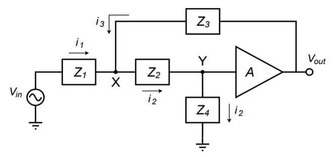
At this point, we need to derive the general transfer equation for the circuit. Once the general equation is established, we will be able to refine the circuit for special cases. Being a higher-order active circuit, this procedure will naturally be somewhat more involved than the derivations found in Chapter One for the simple first-order lead and lag networks. The concepts are consistent though. This derivation utilizes a nodal analysis. In order to make the analysis a bit more convenient, it will help if we declare the voltage 𝑉𝑦 as 1 V. This will save us from carrying an input voltage factor through our calculations, which would need to be factored out of the general equation anyway. By inspection we note the following:
![\[V_{out} = AV_y = A \]](https://pressbooks.nscc.ca/app/uploads/quicklatex/quicklatex.com-45fe9a6945beb482e27f74b2f2afc2c8_l3.png "Rendered by QuickLaTeX.com")
(11.6.1)
![\[i_1 = \frac{V_{in} - V_x}{Z_1} \]](https://pressbooks.nscc.ca/app/uploads/quicklatex/quicklatex.com-9ecb6c952e24c6d973e967dbfb89d204_l3.png "Rendered by QuickLaTeX.com")
![\[i_2 = \frac{1}{Z_4} \]](https://pressbooks.nscc.ca/app/uploads/quicklatex/quicklatex.com-26a45e19a59e5ca67c35c00c538552de_l3.png "Rendered by QuickLaTeX.com")
(11.6.2)
![\[i_3 = \frac{V_{out} - V_x}{Z_3} = \frac{A - V_x}{Z_3} \]](https://pressbooks.nscc.ca/app/uploads/quicklatex/quicklatex.com-7538c13ffd33bc47c35a419af89083dc_l3.png "Rendered by QuickLaTeX.com")
![\[V_x = i_2 Z_2 + V_y = i_2 Z_2 + 1 \]](https://pressbooks.nscc.ca/app/uploads/quicklatex/quicklatex.com-34e6ee26a05b9b7fbf86bdae40cfee94_l3.png "Rendered by QuickLaTeX.com")
(11.6.3)
By the substituting Equation 11.6.2 into Equation 11.6.3 , 𝑉𝑥 may be expressed as
![\[V_x = \frac{Z_2}{Z_4} +1 \]](https://pressbooks.nscc.ca/app/uploads/quicklatex/quicklatex.com-30cb9583fdbaa521d63b9dd9e69f705e_l3.png "Rendered by QuickLaTeX.com")
We now sum the currents according to the figure,
![\[i_2 = i_1 + i_3 \]](https://pressbooks.nscc.ca/app/uploads/quicklatex/quicklatex.com-9b1c4027f2aec57f3021e3f726e0027b_l3.png "Rendered by QuickLaTeX.com")
substitute our current equivalences,
![\[\frac{1}{Z_4} = \frac{V_{in} - V_x}{Z_1} + \frac{A - V_x}{Z_3} \]](https://pressbooks.nscc.ca/app/uploads/quicklatex/quicklatex.com-81071d53cd513d511dc7c567621f4269_l3.png "Rendered by QuickLaTeX.com")
and solve the equation in terms of 𝑉𝑖𝑛:
![\[\frac{V_{in} − V_x}{Z_1} = \frac{1}{Z_4} − \frac{A − V_x}{Z_3} \]](https://pressbooks.nscc.ca/app/uploads/quicklatex/quicklatex.com-f146a337d7fa0a007e4d4d009866bdb7_l3.png "Rendered by QuickLaTeX.com")
[V_{in} − V_x = \frac{Z_1}{Z_4} − \frac{Z_1 (A − V_x )}{Z_3} \]
[V_{in} = \frac{Z_1}{Z_4} − \frac{Z_1 (A − V_x )}{Z_3} +V_x \]
[V_{in} = \frac{Z_1}{Z_4} − \frac{Z_1 (A − V_x )}{Z_3} + \frac{Z_2}{Z_4} +1 \]
[V_{in} = \frac{Z_1}{Z_4} − \frac{Z_1}{Z_3} \left( A − \frac{Z_2}{Z_4} −1 \right) + \frac{Z_2}{Z_4} +1 \]
[V_{in} = \frac{Z_1}{Z_4} − \frac{Z_1}{Z_3} A+ \frac{Z_1 Z_2} {Z_3 Z_4} + \frac{Z_1}{Z_3} + \frac{Z_2}{Z_4} +1 \] (11.6.4)
We can now write our general transfer equation using Equations 11.6.1 and 11.6.4 .
![\[\frac{V_{out}}{V_{in}} = \frac{A}{\frac{Z_1}{Z_4} + \frac{Z_1}{Z_3} (1 - A) + \frac{Z_1 Z_2}{Z_3 Z_4} + \frac{Z_2}{Z_4} +1} \]](https://pressbooks.nscc.ca/app/uploads/quicklatex/quicklatex.com-84748ca43a015ee0de7338bf7cfac70d_l3.png "Rendered by QuickLaTeX.com")
(11.6.5)
Equation 11.6.5 is applicable to any variation on Figure 11.6.1 that we wish to make. All we need to do is substitute the appropriate circuit elements for 𝑍1 through 𝑍4 . As you might guess, direct substitution of resistance and reactance values would make for considerable work. In order to alleviate this difficulty, designers rely on the Laplace transform technique. This is also known as the 𝑠 domain technique. A detailed analysis of the Laplace transform is beyond the scope of this text, but some familiarity will prove helpful. The basic idea is to replace complex terms with simpler ones. This is performed by setting the variable 𝑠 equal to 𝑗𝜔 . As you will see, this substitution leads to far simpler and more generalized circuit derivations and equations. A capacitive reactance may be reduced as follows.
![\[\text{Capacitive Reactance } = - j X_C \]](https://pressbooks.nscc.ca/app/uploads/quicklatex/quicklatex.com-a7203a214fc1d79b0ec10af510703668_l3.png "Rendered by QuickLaTeX.com")
![\[\text{Capacitive Reactance } = \frac{-j}{\omega C} \]](https://pressbooks.nscc.ca/app/uploads/quicklatex/quicklatex.com-efef2f0ced325165fb19c68834ba1c7a_l3.png "Rendered by QuickLaTeX.com")
![\[\text{Capacitive Reactance } = \frac{1}{j\omega C} \]](https://pressbooks.nscc.ca/app/uploads/quicklatex/quicklatex.com-cf0312b95cf09289b9e6d6df6d23a80e_l3.png "Rendered by QuickLaTeX.com")
![\[\text{Capacitive Reactance } = \frac{1}{sC} \]](https://pressbooks.nscc.ca/app/uploads/quicklatex/quicklatex.com-3ef3b12f36fd41eea20de1215863aae3_l3.png "Rendered by QuickLaTeX.com")
Therefore, whenever a capacitive reactance is needed, the expression 1/𝑠𝐶 is used. Equations can then be manipulated using basic algebra.
Sallen and Key Low-Pass Filters
Let’s derive a general expression based on Equation 11.6.5 for low-pass filters. A low-pass filter is a lag network, so to echo this, we will use resistors for the first two elements and capacitors for the third and forth. Using the 𝑠 operator we find, 𝑍1=𝑅1 , 𝑍2=𝑅2,𝑍3=1/𝑠𝐶1 , and 𝑍4=1/𝑠𝐶2 .
![\[\frac{V_{out}}{V_{in}} = \frac{A}{sR_1C_2+s R_1C_1 (1-A)+s^2 R_1 R_2C_1C_2+s R_2C_2+1} \]](https://pressbooks.nscc.ca/app/uploads/quicklatex/quicklatex.com-7b61776ef5b4d2831077e025b40f92e7_l3.png "Rendered by QuickLaTeX.com")
![\[\frac{V_{out}}{V_{in}} = \frac{A}{s^2 R_1 R_2C_1C_2+s(R_1C_2+R_2C_2+R_1C_1 (1-A))+1} \]](https://pressbooks.nscc.ca/app/uploads/quicklatex/quicklatex.com-2f8dd4f88683747fdc53758e0f5aec9e_l3.png "Rendered by QuickLaTeX.com")
The highest power of 𝑠 in the denominator determines the number of poles in the filter. Because this is a 2 here, the filter must be a 2 pole-type (second-order), as expected. Usually, it is most convenient if the denominator coefficient for 𝑠2 is unity. This makes the equation easier to factor.
![\[\frac{V_{out}}{V_{in}} = \frac{A/R_1R_2C_1C_2}{s^2+s( \frac{1}{R_2C_1} + \frac{1}{R_1C_1} + \frac{1}{R_2C_2} (1-A)) + \frac{1}{R_1R_2C_1C_2}} \]](https://pressbooks.nscc.ca/app/uploads/quicklatex/quicklatex.com-513a5e9e7167cd4329328005b5a8c064_l3.png "Rendered by QuickLaTeX.com")
(11.6.6)
Second-order systems appear in a variety of areas including mechanical, acoustical, hydraulic, and electrical. They have been widely studied, and a generalized form of one group of second-order responses is given by
![\[G = \frac{A\omega^2}{s^2+\alpha\omega s + \omega^2} \]](https://pressbooks.nscc.ca/app/uploads/quicklatex/quicklatex.com-0f9437f12d53f2b6cd72b5084a99216e_l3.png "Rendered by QuickLaTeX.com")
(11.6.7)
where 𝐴 is the gain of the system, 𝜔 is the resonant frequency in radians, and 𝛼 is the damping factor.
By comparing the general form of Equation 11.6.7 to the low-pass filter Equation 11.6.6 , we find that
![\[\omega^2 = \frac{1}{R_1 R_2C_1C_2} \]](https://pressbooks.nscc.ca/app/uploads/quicklatex/quicklatex.com-f515587ccb72fe0e8c57c8bcba6529f2_l3.png "Rendered by QuickLaTeX.com")
(11.6.8)
![\[\alpha\omega = \frac{1}{R_2C_1} + \frac{1}{R_1C_1} + \frac{1}{R_2C_2} (1-A) \]](https://pressbooks.nscc.ca/app/uploads/quicklatex/quicklatex.com-dc94dcd33774f05e2243d0d4062bc838_l3.png "Rendered by QuickLaTeX.com")
(11.6.9)
Based on the general expression of Equation 11.6.7 , we can derive equations for the gain magnitude versus frequency and phase versus frequency, as we did in Chapter One for the first-order systems. For most filter work, it is convenient to work with normalized frequency instead of a true frequency. This means that the critical frequency will be set to 1 radian per second, and a generalized equation developed. For circuits using other critical frequencies, the general equation is used and its results are simply scaled by a factor equal to this new frequency. The normalized version of Equation 11.6.7 is
![\[G = \frac{A}{s^2 + \alpha s + 1} \]](https://pressbooks.nscc.ca/app/uploads/quicklatex/quicklatex.com-738a1f2967b60fe77224b6ffd54c8949_l3.png "Rendered by QuickLaTeX.com")
(11.6.10)
In order to determine the gain and phase expressions, Equation 11.6.10 must be split into its real and imaginary components. The first step is to replace 𝑠 with its equivalent, 𝑗𝜔 , and then group the real and imaginary components.
![\[G = \frac{A}{( j\omega)^2 + j \alpha\omega+1} \]](https://pressbooks.nscc.ca/app/uploads/quicklatex/quicklatex.com-c557db3b24c823f4e65375c1e0f7a8bc_l3.png "Rendered by QuickLaTeX.com")
![\[G = \frac{A}{-\omega^2 + j\alpha\omega+1} \]](https://pressbooks.nscc.ca/app/uploads/quicklatex/quicklatex.com-755a470ab7d15d13db5b924715106fbd_l3.png "Rendered by QuickLaTeX.com")
![\[G = \frac{A}{(1-\omega^2 ) + j\alpha \omega} \]](https://pressbooks.nscc.ca/app/uploads/quicklatex/quicklatex.com-1e9e7e8a2e42511ed4a1c91a403f9726_l3.png "Rendered by QuickLaTeX.com")
To split this into separate real and imaginary components, we must multiply the numerator and denominator by the complex conjugate of the denominator, (1−𝜔2)−𝑗𝛼𝜔 .
![\[G = \frac{A}{(1−\omega^2 ) + j\alpha\omega}\frac{(1−\omega^2 ) − j \alpha\omega}{(1−\omega^2 )− j \alpha\omega} \]](https://pressbooks.nscc.ca/app/uploads/quicklatex/quicklatex.com-0e96329e328db438c272faad9c9f7c75_l3.png "Rendered by QuickLaTeX.com")
[G = \frac{A((1−\omega^2 ) − j \alpha\omega)}{(1−\omega^2 )^2+\alpha^2 \omega^2} \]
Applying Equation 11.6.11 to this relation yields
![\[\text{Mag } = \sqrt{\left( \frac{A(1-\omega^2 )}{(1-\omega^2 )^2+\alpha^2 \omega^2} \right)^2 + \left( - \frac{A\alpha\omega}{(1 - \omega^2 )^2+\alpha^2\omega^2} \right)^2} \]](https://pressbooks.nscc.ca/app/uploads/quicklatex/quicklatex.com-6df3027ccd13161e4f33dfe7c0435eee_l3.png "Rendered by QuickLaTeX.com")
![\[ \text{Mag } = \sqrt{ \frac{A^2 (1-\omega^2 )^2}{((1-\omega^2 )^2 + \alpha^2 \omega^2 )^2} + \frac{A^2 \alpha^2 \omega^2}{((1-\omega^2 )^2 + \alpha^2 \omega^2 )^2}} \]](https://pressbooks.nscc.ca/app/uploads/quicklatex/quicklatex.com-1ce6d22e5cd2912da9df6f432194b9e9_l3.png "Rendered by QuickLaTeX.com")
![\[ \text{Mag } = \frac{\sqrt{A^2 ((1−\omega^2 )^2+\alpha^2\omega^2 )}}{((1-\omega^2 )^2+\alpha^2 \omega^2 )^2} \]](https://pressbooks.nscc.ca/app/uploads/quicklatex/quicklatex.com-3198a3f3146b73cbf9ec678a0f3ae682_l3.png "Rendered by QuickLaTeX.com")
![\[ \text{Mag } = \frac{A \sqrt{(1-\omega^2 )^2+\alpha^2 \omega^2}}{(1-\omega^2 )^2+\alpha^2 \omega^2} \]](https://pressbooks.nscc.ca/app/uploads/quicklatex/quicklatex.com-07b8b70a2af3e0c0f7de4a3ad78ddaf8_l3.png "Rendered by QuickLaTeX.com")
![\[ \text{Mag } = \frac{A}{\sqrt{(1-\omega^2 )^2+\alpha^2 \omega^2}} \]](https://pressbooks.nscc.ca/app/uploads/quicklatex/quicklatex.com-8119aace86bf7a794d8a2a6bdeeb8bad_l3.png "Rendered by QuickLaTeX.com")
(11.6.12)
For the phase response, recall that 𝜃=tan−1(𝑖𝑚𝑎𝑔𝑖𝑛𝑎𝑟𝑦/𝑟𝑒𝑎𝑙) . Applying Equation 11.6.11 to this relation yields
![\[\theta = \arctan \frac{- \frac{A\alpha\omega}{(1-\omega^2 )^2 + \alpha^2 \omega^2}}{\frac{A(1-\omega^2 )}{ (1-\omega^2 )^2 + \alpha^2 \omega^2}} \]](https://pressbooks.nscc.ca/app/uploads/quicklatex/quicklatex.com-f752d021cae588c9f726621a618b89dd_l3.png "Rendered by QuickLaTeX.com")
![\[ \theta = \arctan \frac{-A\alpha\omega}{A(1-\omega^2 )} \]](https://pressbooks.nscc.ca/app/uploads/quicklatex/quicklatex.com-e71313a1fd6f840400c938dbe76ec8fa_l3.png "Rendered by QuickLaTeX.com")
(11.6.13)
To use Equations 11.6.12 and 11.6.13 with a particular alignment, substitute the appropriate damping value and simplify. Derivation of specific damping factors is beyond the scope of this chapter, but can be found in texts specializing on filter design. For our purposes, tables of damping factors for specific alignments will be presented. As one possible example, the damping factor for a second-order Butterworth alignment is 2‾√ . Substituting this into Equation 11.6.12 produces
![\[\text{Mag } = \frac{A}{\sqrt{1+\omega^2 (\alpha^2 - 2) + \omega^4}} \]](https://pressbooks.nscc.ca/app/uploads/quicklatex/quicklatex.com-4460edc6b8a041a917dc3e235b108729_l3.png "Rendered by QuickLaTeX.com")
![\[\text{Mag } = \frac{A}{\sqrt{1+\omega^2 ((\sqrt{2})^2 -2) + \omega^4}} \]](https://pressbooks.nscc.ca/app/uploads/quicklatex/quicklatex.com-494914e39b807da3217f25a2ce87bc87_l3.png "Rendered by QuickLaTeX.com")
![\[\text{Mag } = \frac{A}{\sqrt{1 + \omega^4}} \]](https://pressbooks.nscc.ca/app/uploads/quicklatex/quicklatex.com-873e7fb04dce4aee88e1e394a613bd78_l3.png "Rendered by QuickLaTeX.com")
There are a large number of ways of configuring a low-pass filter given the above equations. So that we might put some consistency into what appears to be a chaotic mess, we’ll look at two distinct and useful variations. They are the equal component realization and the unity gain realization.
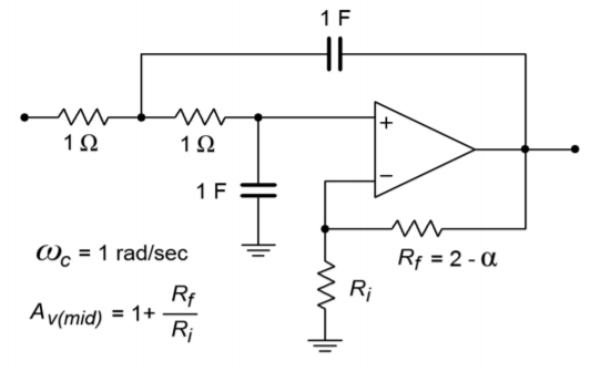
The equal-component version
Here, we will set 𝑅1=𝑅2 and 𝐶1=𝐶2 . To keep the resulting equation generic, we will use a normalized frequency of 1 radian per second. For other tuning frequencies, we will just scale our results to the desired value. From Equation 11.6.8 , if 𝜔=1 , then 𝑅1𝑅2𝐶1𝐶2=1 , and the most straightforward solution would be to set 𝑅1=𝑅2=𝐶1=𝐶2=1 (units of ohms and farads). Equation 11.6.6 simplifies to
![\[\frac{V_{out}}{V_{in}} = \frac{A}{s^2 + s(1+1+1(1 -A))+1} \]](https://pressbooks.nscc.ca/app/uploads/quicklatex/quicklatex.com-d7d9c6fb2705095b7cb654af4d490ec9_l3.png "Rendered by QuickLaTeX.com")
Note the damping factor is now given by
![\[\alpha = 1+1+1(1-A) \]](https://pressbooks.nscc.ca/app/uploads/quicklatex/quicklatex.com-dc278ab8f90a911c8450dd6e7d455579_l3.png "Rendered by QuickLaTeX.com")
![\[\alpha = 3 - A \]](https://pressbooks.nscc.ca/app/uploads/quicklatex/quicklatex.com-6fd69f78c1af34ce716f89963b5528e8_l3.png "Rendered by QuickLaTeX.com")
We see that the gain and damping of the filter are linked together. Indeed, for a certain damping factor, only one specific gain will work properly:
![\[A = 3 - \alpha \]](https://pressbooks.nscc.ca/app/uploads/quicklatex/quicklatex.com-ddd7960abca642d3df77529e31a7b879_l3.png "Rendered by QuickLaTeX.com")
As the gain of a noninverting amplifier is
![\[A = 1 + \frac{R_f}{R_i} \]](https://pressbooks.nscc.ca/app/uploads/quicklatex/quicklatex.com-bf69d6a803091388e1c38cd76efa8ee0_l3.png "Rendered by QuickLaTeX.com")
we may find the required value for 𝑅𝑓 by combining these two equations:
![\[R_f = 2 - \alpha \]](https://pressbooks.nscc.ca/app/uploads/quicklatex/quicklatex.com-2bc8ba04ebf902d89832ad008851307f_l3.png "Rendered by QuickLaTeX.com")
The finished prototype is shown in Figure 11.6.2 .
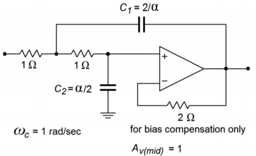
The unity-gain version
Here we will set 𝐴=1 , and 𝑅1=𝑅2 . From Equation 11.6.8 , if 𝜔=1 , then 𝑅1𝑅2𝐶1𝐶2=1 , and therefore 𝐶1=1/𝐶2 . In effect, the ratio of the capacitors will set the damping factor for the system. Equation 11.6.6 may be simplified to
![\[\frac{V_{out}}{V_{in}} = \frac{A}{s^2 + s( \frac{1}{C_1} + \frac{1}{C_1} ) + 1} \]](https://pressbooks.nscc.ca/app/uploads/quicklatex/quicklatex.com-1439c70a61dad51f6f248e23dccca947_l3.png "Rendered by QuickLaTeX.com")
The damping factor is now given by
![\[\alpha = \frac{1}{C_1} + \frac{1}{C_1} \]](https://pressbooks.nscc.ca/app/uploads/quicklatex/quicklatex.com-975f824beaae3a057d21c57394e8ca03_l3.png "Rendered by QuickLaTeX.com")
![\[ \alpha = \frac{2}{C_1} \text{ or,} \]](https://pressbooks.nscc.ca/app/uploads/quicklatex/quicklatex.com-7d26fcc575a33b8c174e473a219c7c60_l3.png "Rendered by QuickLaTeX.com")
![\[ C_1 = \frac{2}{\alpha} \]](https://pressbooks.nscc.ca/app/uploads/quicklatex/quicklatex.com-fdd0be12e75ec0102a6a1f0ed71a0cd1_l3.png "Rendered by QuickLaTeX.com")
Because 𝐶1=1/𝐶2 , we find
![\[C_2 = \frac{\alpha}{2} \]](https://pressbooks.nscc.ca/app/uploads/quicklatex/quicklatex.com-09805dcb4407bf85305b40c652fe6ddf_l3.png "Rendered by QuickLaTeX.com")
The finished prototype is shown in Figure 11.6.3 .
As you can see, there is quite a bit of similarity between the two versions. It is important to note that the inputs to these circuits must return to ground via a low-impedance DC path. If the signal source is capacitively coupled, the op amp’s input bias current cannot be set up properly, and thus, some form of DC return resistor must be used at the source. Also, you can see that the damping factor (i.e., alignment) of the filter plays a role in setting component values. If the values shown are taken as having units of ohms and farads, the critical frequency will be 1 radian per second. It is an accepted practice to normalize the basic forms of circuits such as these, so that the critical frequency works out to this convenient value. This makes it very easy to scale the component values to fit your desired critical frequency. Because the critical frequency is inversely proportional to the tuning resistor and capacitor values, you only need to shrink 𝑅 or 𝐶 in order to increase 𝑓𝑐 . (Remember, 𝑓𝑐=1/(2𝜋𝑅𝐶)) . A second scaling step normally follows this, in order to create practical values for 𝑅 and 𝐶 . This procedure is best shown with an example.
Example 11.6.1
Design a 1 kHz low-pass, second-order Butterworth filter. Examine both the equal-component and the unity-gain forms as drawn in Figure 11.6.2 and 11.6.3 , respectively. The required damping factor is 1.414.
Let’s start with the equal-component version. First, find the required value for 𝑅𝑓 from the damping factor, as given on the diagram.
![\[R_f = 2 - \alpha \\ R_f = 2 −1.414 \]](https://pressbooks.nscc.ca/app/uploads/quicklatex/quicklatex.com-15ed66fe3cef7bb389a0c61f1e6ed339_l3.png "Rendered by QuickLaTeX.com")
[
![\[R_f = 0.586\Omega \nonumber \]](https://pressbooks.nscc.ca/app/uploads/quicklatex/quicklatex.com-94914168455314b6997f9ad418f58c70_l3.png "Rendered by QuickLaTeX.com")
Note that this will produce a pass-band gain of
![\[A_v = 1+ \frac{R_f}{R_i} \]](https://pressbooks.nscc.ca/app/uploads/quicklatex/quicklatex.com-3fead3440157629d6ec728f5898786be_l3.png "Rendered by QuickLaTeX.com")
![\[ A_v = 1+ \frac{0.586}{1} \]](https://pressbooks.nscc.ca/app/uploads/quicklatex/quicklatex.com-8676cb0a1d56302ded6486a43cb8c144_l3.png "Rendered by QuickLaTeX.com")
![\[ A_v = 1.586 \]](https://pressbooks.nscc.ca/app/uploads/quicklatex/quicklatex.com-74e7bdde938f863fa7e665e00ce71bfa_l3.png "Rendered by QuickLaTeX.com")

Figure 11.6.4 shows the second-order Butterworth low-pass filter. Its critical frequency is 1 radian per second. We need to scale this to 1 kHz.
![\[\omega_c = 2\pi f_c \]](https://pressbooks.nscc.ca/app/uploads/quicklatex/quicklatex.com-282576a9c19f641acf2ac8e9a028ac0a_l3.png "Rendered by QuickLaTeX.com")
![\[ \omega_c = 2\pi 1 kHz \]](https://pressbooks.nscc.ca/app/uploads/quicklatex/quicklatex.com-5f9f64005e8437b57913fa41df72edaf_l3.png "Rendered by QuickLaTeX.com")
![\[ \omega_c = 6283 \text{ radians per second} \]](https://pressbooks.nscc.ca/app/uploads/quicklatex/quicklatex.com-361aee56cb472e09d8d46933684df9d7_l3.png "Rendered by QuickLaTeX.com")
Our desired critical frequency is 6283 times higher than the normalized base. As 𝜔𝑐=1/𝑅𝐶 , to translate the frequency up, all we need to do is divide 𝑅 or 𝐶 by 6283. It doesn’t really matter which one you choose, although it is generally easier to find “odd” sizes for resistors than capacitors, so we’ll use 𝑅 .
![\[R = \frac{1}{6283} \]](https://pressbooks.nscc.ca/app/uploads/quicklatex/quicklatex.com-ad9e8bf34fbfc46efc6f1726e9dfe74c_l3.png "Rendered by QuickLaTeX.com")
![\[ R = 1.59 \times 10^{-4} \Omega \]](https://pressbooks.nscc.ca/app/uploads/quicklatex/quicklatex.com-a9d7938fb70b5f43106a22ae17fddd36_l3.png "Rendered by QuickLaTeX.com")
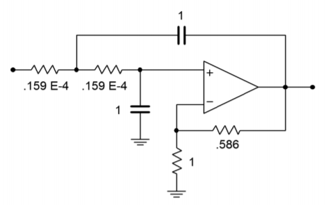
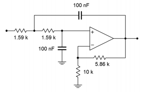
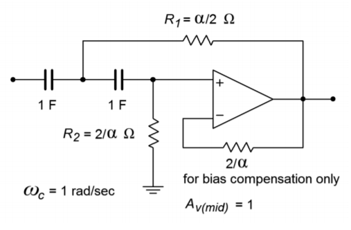
Figure 11.6.5 shows our 1 kHz, low-pass, second-order Butterworth filter. As you can see, though, the component values are not very practical. It is therefore necessary to perform the final scaling operations. First, consider multiplying 𝑅𝑓 and 𝑅𝑖 by 10 k. Note that this will have no effect on the damping, as it is the ratio of these two elements that determines damping. This scaling will not affect the critical frequency either, as 𝑓𝑐 is set by the tuning resistors and capacitors. Second, we need to increase 𝑅 to a reasonable value. A factor of 107 will place it at 1.59𝑘Ω . In order to compensate, the tuning capacitors must be dropped by an equal amount, which brings them to 100 nF. The completed design is shown in Figure 11.6.6 . Other scaling factors could also be used. Also, if bias compensation is important, the 𝑅𝑖 and 𝑅𝑓 values will need to be scaled further, in order to balance the resistance seen at the noninverting input.
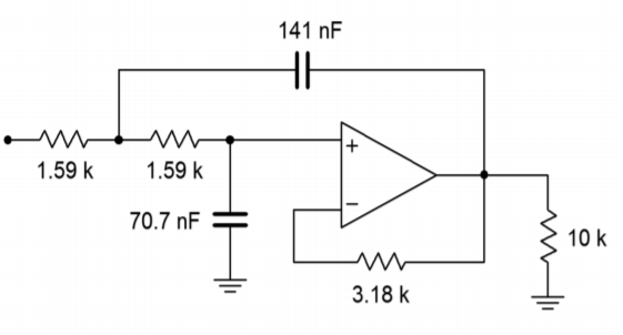
The approach for the unity-gain version is similar. First, adjust the capacitor values in order to achieve the desired damping, as specified in Figure 11.6.3 .
![\[C_1 = \frac{2}{\alpha} \]](https://pressbooks.nscc.ca/app/uploads/quicklatex/quicklatex.com-40223512768facac2aa94cb19f75387f_l3.png "Rendered by QuickLaTeX.com")
![\[ C_1 = \frac{2}{1.414} \]](https://pressbooks.nscc.ca/app/uploads/quicklatex/quicklatex.com-8034ae688ff108cfe47590c4330394d9_l3.png "Rendered by QuickLaTeX.com")
![\[ C_1 = 1.414 F \]](https://pressbooks.nscc.ca/app/uploads/quicklatex/quicklatex.com-79d454872687a1d40d75c22aa1d002f4_l3.png "Rendered by QuickLaTeX.com")
![\[ C_2 = \frac{1.414}{2} \]](https://pressbooks.nscc.ca/app/uploads/quicklatex/quicklatex.com-209eeb9450f73e5a43e9fd943bbda0a3_l3.png "Rendered by QuickLaTeX.com")
![\[ C_2 = 0.707 F \]](https://pressbooks.nscc.ca/app/uploads/quicklatex/quicklatex.com-d23a4b9cd0eb619d914cb34234ce2746_l3.png "Rendered by QuickLaTeX.com")
The resulting circuit is shown in Figure 11.6.7 . The circuit must be scaled to the desired 𝑓𝑐 . The factor is 6283 once again, and the result is shown in Figure 11.6.8 . The final component scaling is seen in Figure 11.6.9 .


Computer Simulation
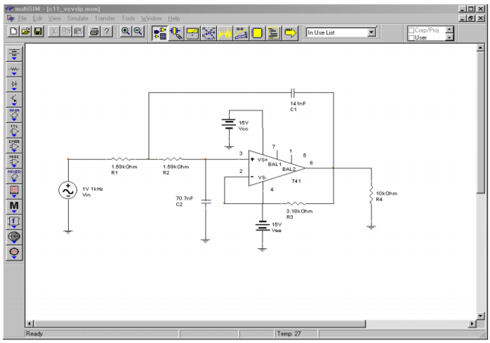
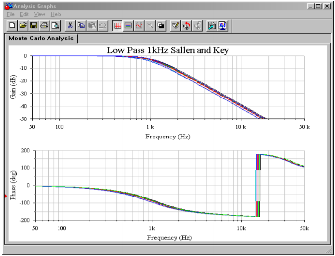
A Multisim simulation of the filter design of Example 11.6.1 is shown in Figure 11.6.10 . The analysis shows the Bode plot, ranging from 50 Hz to better than 20 kHz. This yields over one decade on either side of the 1 kHz critical frequency. The graph clearly shows the −3 dB point at approximately 1 kHz, with an attenuation slope of −12 dB per octave. Since this is the unity-gain version, the low-frequency gain is set at 0 dB. Also, note that no peaking is evident in the response curve, as is expected for a Butterworth alignment. The phase response is also shown. Some graphing tools continue the phase shift below −180 degrees, whereas others will flip it back to +180, as Multisim does. Note that if the frequency plot range is extended, the phase shift starts to increase at the highest frequencies instead of leveling off. This is due to the extra phase shift produced by the op amp as the operating frequency approaches 𝑓𝑢𝑛𝑖𝑡𝑦 . A simpler op amp model would not create this real-world effect.

Finally, a Monte Carlo analysis is used to mimic the effects seen due to component tolerance in a production environment (in this example, approximately 10 percent variation of nominal for each component). A total of 10 runs were generated. Although the overall shape of the curve remains consistent, there is some variation in the corner frequency, certainly more than the 10 percent offered by any single component. As you might guess, a Monte Carlo analysis is very tedious to do by hand, but quite straightforward to set up on a simulator.
As you can see, the realization process is little more than a scaling sequence. This makes filter design very rapid. The operation for high-pass filters is essentially the same.
Sallen and Key High-Pass Filters
We can derive a general expression for high-pass filters, based on Equation 11.6.5 . A high-pass filter is a lead network, so to echo this, we will use capacitors for the first two elements and resistors for the third and forth. Using the 𝑠 operator, we find, 𝑍1=1/𝑠𝐶1 , 𝑍2=1/𝑠𝐶2 , 𝑍3=𝑅1 , and 𝑍4=𝑅2 .
![\[\frac{V_{out}}{V_{in}} = \frac{A}{\frac{Z_1}{Z_4} + \frac{Z_1}{Z_3} (1-A)+ \frac{Z_1Z_2}{Z_3Z_4} + \frac{Z_2}{Z_4} +1} \]](https://pressbooks.nscc.ca/app/uploads/quicklatex/quicklatex.com-bb5209b3a1fe7defaa6b9f9acbf0f1b8_l3.png "Rendered by QuickLaTeX.com")
![\[ \frac{V_{out}}{V_{in}} = \frac{A}{\frac{1}{s R_2C_1} + \frac{1}{s R_1C_1} (1-A) + \frac{1}{s^2 R_1 R_2C_1C_2} + \frac{1}{s R_2C_2} +1} \]](https://pressbooks.nscc.ca/app/uploads/quicklatex/quicklatex.com-7d7e6ee761e852a98047694417dd6401_l3.png "Rendered by QuickLaTeX.com")
![\[\frac{V_{out}}{V_{in}} = \frac{A s^2}{s^2+s( \frac{1}{R_2C_1} + \frac{1}{R_2C_2} + \frac{1}{R_1C_1} (1−A)) + \frac{1}{R_1R_2C_1C_2}} \]](https://pressbooks.nscc.ca/app/uploads/quicklatex/quicklatex.com-e5e9b09e6278bb47cba22a25aab7525f_l3.png "Rendered by QuickLaTeX.com")
(11.6.14)
As with the low-pass filters we have two basic realizations: equal-component and unity-gain. In both cases, we start with Equation 11.6.14 and use normalized frequency (1 radian per second). The derivations are very similar to the low-pass case, and the results are summarized below. The equal-component version:
![\[\alpha = 3 -A \]](https://pressbooks.nscc.ca/app/uploads/quicklatex/quicklatex.com-b7336e95b654829bd9f49d811c16031e_l3.png "Rendered by QuickLaTeX.com")
The unity-gain version:
![\[R_2 = \frac{2}{\alpha} \]](https://pressbooks.nscc.ca/app/uploads/quicklatex/quicklatex.com-210817abe034bc8e12acb6810361c5ad_l3.png "Rendered by QuickLaTeX.com")
![\[ R_1 = \frac{\alpha}{2} \]](https://pressbooks.nscc.ca/app/uploads/quicklatex/quicklatex.com-b986e3f6868170a6007873219eb4977d_l3.png "Rendered by QuickLaTeX.com")
These forms are shown in Figures Figure 11.6.11 and Figure 11.6.12 . You may at this point ask two questions: One, how do you find the damping factor, and two, what about higher-order filters?
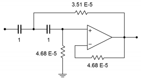
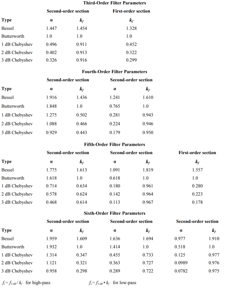
In order to find the damping factor needed, a chart such as Figure Figure 11.6.13 may be consulted. This chart also introduces a new item, and that is the frequency factor, 𝑘𝑓 . Normally, the critical frequency and 3 dB down frequency (break frequency) of a filter are not the same value. They are identical only for the Butterworth alignment.
For any other alignment, the desired break frequency must first be translated to the appropriate critical frequency before scaling is performed. This is illustrated in the following example.

Example 11.6.2
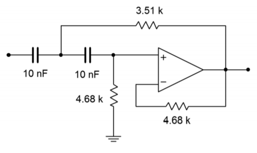
Design a second-order, high-pass Bessel filter, with a break frequency (𝑓3𝑑𝐵) of 5 kHz.
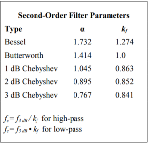
For this example, let’s use the unity-gain form shown in Figure Figure 11.6.11 . First, obtain the damping and frequency factors from Figure Figure 11.6.13 .
![\[k_f = 1.274, \text{ damping } = 1.732. \]](https://pressbooks.nscc.ca/app/uploads/quicklatex/quicklatex.com-fc8f7ca28673bdffff17c8b766f1c689_l3.png "Rendered by QuickLaTeX.com")
Using the damping factor, the two tuning resistors may be found:
![\[R_1 = \frac{\alpha}{2} \]](https://pressbooks.nscc.ca/app/uploads/quicklatex/quicklatex.com-f94634291069d8a8a9bf44fefce5d931_l3.png "Rendered by QuickLaTeX.com")
![\[ R_1 = \frac{1.732}{2} \]](https://pressbooks.nscc.ca/app/uploads/quicklatex/quicklatex.com-3ed0dd1d194e74d3223e9efdc6e024ca_l3.png "Rendered by QuickLaTeX.com")
![\[ R_1 = .866\Omega \]](https://pressbooks.nscc.ca/app/uploads/quicklatex/quicklatex.com-0149204b6cc55e36427a5f4ef0e6d707_l3.png "Rendered by QuickLaTeX.com")
![\[ R_2 = \frac{2}{1.732} \]](https://pressbooks.nscc.ca/app/uploads/quicklatex/quicklatex.com-c1d27dfcc1301f136d3160572d72e68a_l3.png "Rendered by QuickLaTeX.com")
![\[ R_2 = 1.155\Omega \]](https://pressbooks.nscc.ca/app/uploads/quicklatex/quicklatex.com-007c9a11f58442c71c18efa1ab6997b7_l3.png "Rendered by QuickLaTeX.com")
The intermediate result is shown in Figure Figure 11.6.14 . In order to do the frequency scaling, the desired break frequency of 5 kHz must first be translated into the required critical frequency. Because this is a high-pass filter,
![\[f_c = \frac{f_{3dB}}{k_f} \]](https://pressbooks.nscc.ca/app/uploads/quicklatex/quicklatex.com-e9c067b25277d760828a4fc2d946e823_l3.png "Rendered by QuickLaTeX.com")
![\[ f_c = \frac{5 kHz}{1.274} \]](https://pressbooks.nscc.ca/app/uploads/quicklatex/quicklatex.com-855c03fb86fe08851d93cdc668bc30f5_l3.png "Rendered by QuickLaTeX.com")
![\[ f_c = 3925 Hz \]](https://pressbooks.nscc.ca/app/uploads/quicklatex/quicklatex.com-5c36668f6f1aee1e77ccb5f58c429e84_l3.png "Rendered by QuickLaTeX.com")
![\[ \omega_c = 2\pi 3925 \]](https://pressbooks.nscc.ca/app/uploads/quicklatex/quicklatex.com-10123439360817eb7b84ee27e29cd7e7_l3.png "Rendered by QuickLaTeX.com")
![\[ \omega_c = 24.66 k \text{ radians per second} \]](https://pressbooks.nscc.ca/app/uploads/quicklatex/quicklatex.com-d1807b4df6f97673fe277f1397d8e243_l3.png "Rendered by QuickLaTeX.com")
Either the tuning resistors or capacitors may now be scaled.
![\[R_1 = \frac{.866}{24.66 k} \]](https://pressbooks.nscc.ca/app/uploads/quicklatex/quicklatex.com-00200606126d933c0bda9d21aa662413_l3.png "Rendered by QuickLaTeX.com")
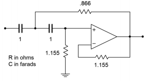
![\[ R_1 = 3.51 \times 10^{-5} \Omega \]](https://pressbooks.nscc.ca/app/uploads/quicklatex/quicklatex.com-b23a38adbc79b728ef197f89a0385a16_l3.png "Rendered by QuickLaTeX.com")
![\[R_2 = \frac{1.155}{24.66 k} \]](https://pressbooks.nscc.ca/app/uploads/quicklatex/quicklatex.com-c550101722f00743dca3ef5073a96980_l3.png "Rendered by QuickLaTeX.com")
![\[ R_2 = 4.68 \times 10^{-5} \Omega \]](https://pressbooks.nscc.ca/app/uploads/quicklatex/quicklatex.com-975853ab5276018ead92f6f3b183f575_l3.png "Rendered by QuickLaTeX.com")
We now have a second-order, high-pass, 5 kHz Bessel filter. This is shown in Figure Figure 11.6.15 . A final scaling of 108 will give us reasonable values, and is shown in Figure Figure 11.6.16 .
Filters of Higher Order
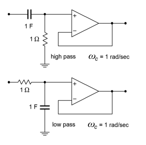
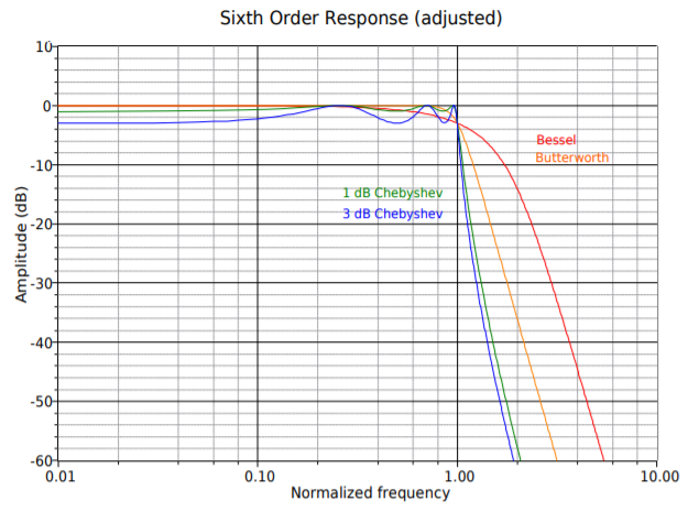
There is a common misconception among novice filter designers that higher-order filters may be produced by cascading a number of lower-order filters of the same type. This is not true. For example, cascading three second-order 10 kHz Butterworth filters will not} produce a sixth-order 10 kHz Butterworth filter. A quick inspection reveals why this is not the case: A single filter of any order will show a 3 dB loss at its break frequency by definition (in this case, 10 kHz). If three filters of the same type are cascaded, each filter will produce a 3 dB loss at the break frequency, which means an overall loss of 9 dB occurs. This much is true: a higher order filter will require a number of individual sections, each with specific damping and frequency factors. Each section will be based on the second-order forms already examined.[1] In order to make odd-ordered filters, we will introduce a simple single-pole filter. The high- and low-pass versions of this unit are shown in Figure Figure 11.6.17 . The damping factor for this circuit is always unity. When working with it, you need only worry about the frequency factor.
Designing higher-order filters is, conceptually, no different than designing second-order filters. The reality is that new charts are needed for the required damping and frequency factors. A set of compatible charts is shown in Figure Figure 11.6.18 for orders 3 through 6 on the following pages. An example is then presented to show the design sequence flow.


Example 11.6.3
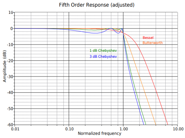
We wish to design a filter suitable for removing subsonic tones from a stereo system. This could be used to reduce turntable rumble in a vintage hi-fi or DJ system, or to reduce stage vibration in a public address system. The filter should attenuate frequencies below the lower limit of human hearing (about 20 Hz), while allowing all higher frequencies to pass. Transient response may be important here, so we’ll choose a Bessel alignment. We will also specify a fifth-order system. This will create an attenuation of about 15 dB, one octave below the break frequency.
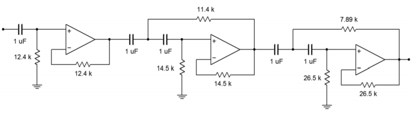
First, note that the specification requires the use of a high-pass filter. This filter may be realized with either the equal-component or the unity-gain forms. As this design will require multiple sections, excessive gain may result from the equal-component version. Our fifth-order system will be comprised of two second-order sections and a first-order section. An overview of the design is shown in Figure 11.6.19 , with the appropriate damping and frequency factors taken from Figure 11.6.18 . We’ll break the analysis down stage by stage.

First, find the desired break frequency in radians.
![\[\omega_{3dB} = 2 \pi f_{3dB} \]](https://pressbooks.nscc.ca/app/uploads/quicklatex/quicklatex.com-4fc23578f4664ff579aca5c507bad87f_l3.png "Rendered by QuickLaTeX.com")
![\[ \omega_{3dB} = 2 \pi 20 Hz \]](https://pressbooks.nscc.ca/app/uploads/quicklatex/quicklatex.com-5545215c529a270e3edf41b914a77857_l3.png "Rendered by QuickLaTeX.com")
![\[ \omega_{3dB} = 125.7 \text{ radians per second} \]](https://pressbooks.nscc.ca/app/uploads/quicklatex/quicklatex.com-b0481f2ae4f1b8cc31d77a236be7bd4e_l3.png "Rendered by QuickLaTeX.com")
Stage 1:
The break frequency must be translated to the required critical frequency. Because this is a high-pass filter, we need to divide by the frequency factor.
![\[\omega_c = \frac{\omega_{3dB}}{k_f} \]](https://pressbooks.nscc.ca/app/uploads/quicklatex/quicklatex.com-7f1f32b82481a7fe929d58ae07cd2c16_l3.png "Rendered by QuickLaTeX.com")
![\[ \omega_c = \frac{125.7}{1.557} \]](https://pressbooks.nscc.ca/app/uploads/quicklatex/quicklatex.com-871db2a467c5a39917ef07b11dfb4e80_l3.png "Rendered by QuickLaTeX.com")
![\[ \omega_c = 80.7 \text{ radians per second} \]](https://pressbooks.nscc.ca/app/uploads/quicklatex/quicklatex.com-e996c8d98411d1d835dad3b3efe65210_l3.png "Rendered by QuickLaTeX.com")
We will scale the resistor by 80.7 to achieve this tuning frequency.
![\[R = \frac{1}{80.7} \]](https://pressbooks.nscc.ca/app/uploads/quicklatex/quicklatex.com-4f028077d6697fab727b558a2a08280a_l3.png "Rendered by QuickLaTeX.com")
![\[ R = .0124 \Omega \]](https://pressbooks.nscc.ca/app/uploads/quicklatex/quicklatex.com-b2339d76e68e67d04a74e78d068d554c_l3.png "Rendered by QuickLaTeX.com")
The 𝑅 and 𝐶 values must now be scaled for practical values. A factor of 106 would be reasonable. The final result is
![\[ R = 12.4 k \]](https://pressbooks.nscc.ca/app/uploads/quicklatex/quicklatex.com-64174112240d2eb68649075aeed58e34_l3.png "Rendered by QuickLaTeX.com")
![\[ C = 1\mu F \]](https://pressbooks.nscc.ca/app/uploads/quicklatex/quicklatex.com-9424fef556b91836125dfea6f340a7e0_l3.png "Rendered by QuickLaTeX.com")
Stage 2:
First, determine the values for the two resistors from the given damping factor.
![\[ R_1 = \frac{1.775}{2} \]](https://pressbooks.nscc.ca/app/uploads/quicklatex/quicklatex.com-1b59db3a234bf813931993947610cf1b_l3.png "Rendered by QuickLaTeX.com")
![\[ R_1 = 0.8875\Omega \]](https://pressbooks.nscc.ca/app/uploads/quicklatex/quicklatex.com-f4f4a76e3ee75250808c49c1925a8e8d_l3.png "Rendered by QuickLaTeX.com")
[
![\[R_2 = \frac{2}{1.775} \]](https://pressbooks.nscc.ca/app/uploads/quicklatex/quicklatex.com-0080e9390cecd50027cdbcc9f786235a_l3.png "Rendered by QuickLaTeX.com")
![\[ R_2 = 1.127\Omega \]](https://pressbooks.nscc.ca/app/uploads/quicklatex/quicklatex.com-bf4b9f5e4b82a4381ebaf6a17b3a607c_l3.png "Rendered by QuickLaTeX.com")
Now the break frequency must be translated to the required critical frequency.
![\[ \omega_c = \frac{125.7}{1.613} \]](https://pressbooks.nscc.ca/app/uploads/quicklatex/quicklatex.com-5e0acec770ad4a5925f9dbd732c8c47e_l3.png "Rendered by QuickLaTeX.com")
![\[ \omega_c = 77.9 \text{ radians per second} \]](https://pressbooks.nscc.ca/app/uploads/quicklatex/quicklatex.com-3b0525a755df70559e432098b7965a82_l3.png "Rendered by QuickLaTeX.com")
We will scale the resistors by 77.9 to achieve this tuning frequency.
![\[R_1 = \frac{0.8875}{77.9} \]](https://pressbooks.nscc.ca/app/uploads/quicklatex/quicklatex.com-12e40fcda5ac21868a6007ec358042e5_l3.png "Rendered by QuickLaTeX.com")
![\[ R_1 = 0.0114\Omega \]](https://pressbooks.nscc.ca/app/uploads/quicklatex/quicklatex.com-3531ecbba0e22a0a39b63912e9fb97fd_l3.png "Rendered by QuickLaTeX.com")
![\[R_2 = \frac{1.127}{77.9} \]](https://pressbooks.nscc.ca/app/uploads/quicklatex/quicklatex.com-6ec2db5cc17acdfa8ef3fe298dcdf5ef_l3.png "Rendered by QuickLaTeX.com")
![\[R_2 = 0.0145\Omega \nonumber Again, 𝑅 and 𝐶 must be scaled for practical values. A factor of 106 would be reasonable. The final result is 𝑅1=11.4𝑘𝑅2=14.5𝑘𝐶=1𝜇𝐹 Stage 3: First, determine the values for the two resistors from the given damping factor. \[ R_1 = \frac{\alpha}{2} \]](https://pressbooks.nscc.ca/app/uploads/quicklatex/quicklatex.com-32bd6a76a6813aedec2f21bf912a451e_l3.png "Rendered by QuickLaTeX.com")
![\[ R_1 = \frac{1.091}{2} \]](https://pressbooks.nscc.ca/app/uploads/quicklatex/quicklatex.com-254381afe9aa077eba5dc2d19d64c322_l3.png "Rendered by QuickLaTeX.com")
![\[ R_1 = 0.5455\Omega \]](https://pressbooks.nscc.ca/app/uploads/quicklatex/quicklatex.com-ad075cd84604addb9ea4e54087b78dd3_l3.png "Rendered by QuickLaTeX.com")
![\[ R_2 = \frac{2}{1.091} \]](https://pressbooks.nscc.ca/app/uploads/quicklatex/quicklatex.com-5683703eed64fec972aa9aedb6fe1bff_l3.png "Rendered by QuickLaTeX.com")
![\[R_2 = 1.833\Omega \]](https://pressbooks.nscc.ca/app/uploads/quicklatex/quicklatex.com-f665c66702291d459d08354c315e223c_l3.png "Rendered by QuickLaTeX.com")
Now the break frequency must be translated to the required critical frequency.
![\[ \omega_c = \frac{125.7}{1.819} \]](https://pressbooks.nscc.ca/app/uploads/quicklatex/quicklatex.com-371951c6139cbc49e6c40363bc4129b9_l3.png "Rendered by QuickLaTeX.com")
![\[ \omega_c = 69.1 \text{ radians per second} \]](https://pressbooks.nscc.ca/app/uploads/quicklatex/quicklatex.com-d7c4d092e4937210aceed3495252e55a_l3.png "Rendered by QuickLaTeX.com")
We will scale the resistors by 69.1 to achieve this tuning frequency.
![\[R_1 = \frac{.5455}{69.1} \]](https://pressbooks.nscc.ca/app/uploads/quicklatex/quicklatex.com-b5495cc44e4254dd84c3d743f068b7e2_l3.png "Rendered by QuickLaTeX.com")
![\[R_1 = 7.89 \times 10^{-3}\Omega \]](https://pressbooks.nscc.ca/app/uploads/quicklatex/quicklatex.com-2cf1971abf9723cfddda4c69b5e11234_l3.png "Rendered by QuickLaTeX.com")
![\[R_2 = \frac{1.833}{69.1} \]](https://pressbooks.nscc.ca/app/uploads/quicklatex/quicklatex.com-c45519659bf9f8c8c1f42f92e3393ae7_l3.png "Rendered by QuickLaTeX.com")
![\[R_2 = 0.0265\Omega \]](https://pressbooks.nscc.ca/app/uploads/quicklatex/quicklatex.com-d4f157fd064a2004817a32e8066dd9d5_l3.png "Rendered by QuickLaTeX.com")
Again, 𝑅 and 𝐶 must be scaled for practical values. A factor of 106 would be reasonable. The final result is
![\[R_1 = 7.89 k\Omega \]](https://pressbooks.nscc.ca/app/uploads/quicklatex/quicklatex.com-af6190f2175ff09b70b2395253133eb2_l3.png "Rendered by QuickLaTeX.com")
![\[R_2 = 26.5 k\Omega \]](https://pressbooks.nscc.ca/app/uploads/quicklatex/quicklatex.com-0ebe814e216cec5c45558597f71f2c99_l3.png "Rendered by QuickLaTeX.com")
![\[C = 1\mu F \]](https://pressbooks.nscc.ca/app/uploads/quicklatex/quicklatex.com-c7721d0ea6cf36452fc34c324b9cf255_l3.png "Rendered by QuickLaTeX.com")
The complete design is shown in Figure 11.6.20 . Note that all of the capacitors are set at 1𝜇𝐹 . This certainly helps to cut inventory and parts placement
We will complete our discussion of high- and low-pass VCVS filters with the following example.
Example 11.6.4
As mentioned earlier, it is common for loudspeaker systems to rely on passive filters to create their crossover networks. More demanding applications such as recording studio monitoring or large public-address systems (i.e., concert systems) cannot afford the losses associated with passive crossovers.
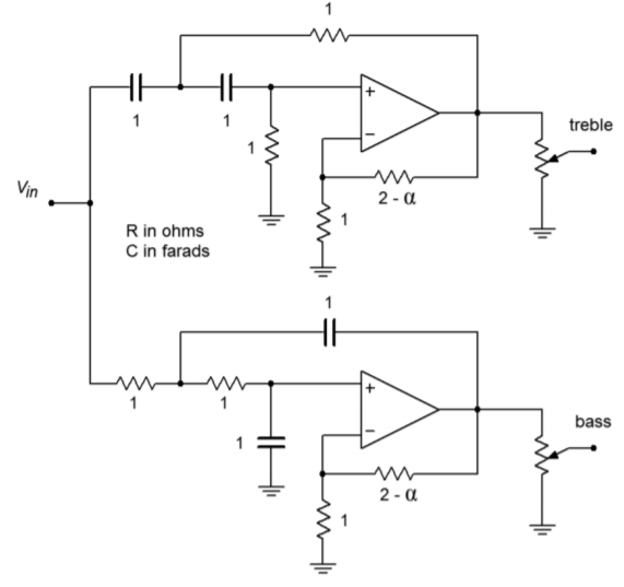
Instead, these applications utilize active crossovers composed of active filters, such as the one shown in Figure 11.6.21 . Before the audio signal is fed to a power amplifier, it is split into two or more frequency bands. The resulting signals each feed their own power amplifier/loudspeaker section.

A block diagram of this approach is shown in Figure 11.6.22 . This one is a two-way system. Large concert sound reinforcement systems may break the audio spectrum into four or five segments. The resulting system will be undoubtedly expensive, but will show lower distortion and higher output levels than a passively-crossed system. A typical two-way system might be crossed at 800 Hz. In other words, frequencies above 800 Hz will be sent to a specialized high frequency-transducer, whereas frequencies below 800 Hz will be sent to a specialized low-frequency transducer. In essence, the crossover network is a combination of an 800 Hz low-pass filter, and an 800 Hz high-pass filter. The filter order and alignment vary considerably depending on the application. Let’s design an 800 Hz crossover with secondorder Butterworth filters.

The basic circuit layout is shown in Figure 11.6.23 . We’re using the equalcomponent value version here. Exact gain is normally not a problem in this case, as some form of volume control needs to be added anyway, in order to compensate between the sensitivity of the low and high frequency transducers. (This is most easily produced by adding a simple voltage divider/potentiometer at the output of the filters.)
For second-order Butterworth filters, the damping factor is found to be 1.414, and the frequency factor is unity (indicating that 𝑓𝑐 and 𝑓3𝑑𝐵 are the same). Note that the design for both halves is almost the same. Both sections show an 𝑓𝑐 of 800 Hz, and a damping factor of 1.414. With identical characteristics, it follows that the component values will be the same in both circuits.
The required value for 𝑅𝑓 is
![\[R_f = 2 − \alpha \]](https://pressbooks.nscc.ca/app/uploads/quicklatex/quicklatex.com-b20529c21a08a0fdbb1edae6d22861de_l3.png "Rendered by QuickLaTeX.com")
![\[R_f = 2 −1.414 \]](https://pressbooks.nscc.ca/app/uploads/quicklatex/quicklatex.com-ca023c5a9e5478c159c3c4458eef6c31_l3.png "Rendered by QuickLaTeX.com")
![\[R_f = 0.586\Omega \]](https://pressbooks.nscc.ca/app/uploads/quicklatex/quicklatex.com-4220a5593656b1d450de5ad5bc21e639_l3.png "Rendered by QuickLaTeX.com")
The critical frequency in radians is
![\[\omega_c = 2\pi 800 Hz \]](https://pressbooks.nscc.ca/app/uploads/quicklatex/quicklatex.com-90266ae45772156662c7a3efbc2967ed_l3.png "Rendered by QuickLaTeX.com")
![\[\omega_c = 5027 \text{ radians per second} \]](https://pressbooks.nscc.ca/app/uploads/quicklatex/quicklatex.com-a601658838726b5e50a3f71f717b912c_l3.png "Rendered by QuickLaTeX.com")
Again, we will scale the tuning resistors to yield
![\[R = \frac{1}{5027} \]](https://pressbooks.nscc.ca/app/uploads/quicklatex/quicklatex.com-51e0d0878205605b0b9476052c17a4ff_l3.png "Rendered by QuickLaTeX.com")
![\[R = 1.989 \times 10^{-4} \Omega \]](https://pressbooks.nscc.ca/app/uploads/quicklatex/quicklatex.com-0dfa2cc11796dbb565dde6bd2f242361_l3.png "Rendered by QuickLaTeX.com")
A final 𝑅𝐶 scaling by 108 produces
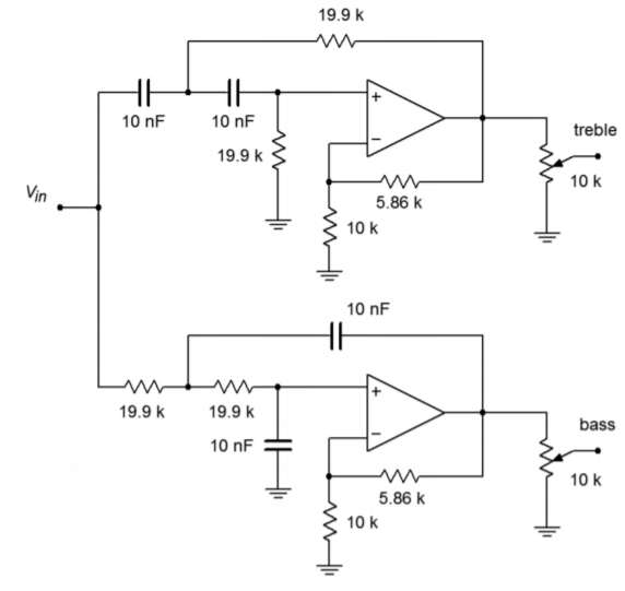
![\[R = 19.9 k\Omega \]](https://pressbooks.nscc.ca/app/uploads/quicklatex/quicklatex.com-19c0676b53ed95a833aa172ffbb8f868_l3.png "Rendered by QuickLaTeX.com")
![\[C = 10 nF \]](https://pressbooks.nscc.ca/app/uploads/quicklatex/quicklatex.com-6a1b3d4f9b848aebc24421b5c1d20411_l3.png "Rendered by QuickLaTeX.com")
𝑅𝑖 and 𝑅𝑓 are scaled by 10𝑘 , and 10𝑘Ω log taper potentiometers may be used for the output volume trimmers. The resulting circuit is shown in Figure 11.6.24 .
- The transfer function of a higher-order filter contains a high-order polynomial in the denominator of the form 𝑠𝑛+𝑏𝑛−1𝑠𝑛−1+⋯+𝑏1𝑠+𝑏0 . The 𝑛 indicates the order of the filter and the 𝑏 coefficients determine the alignment. This polynomial is factored into a product of second-order expressions (with a possible first-order unit for odd-ordered systems). Each of these expressions corresponds to a single section in the larger filter. ↵
