
15.9 Audio Equalizers
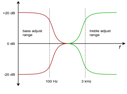
Another range of circuits that fall under the heading of filters are equalizers. Actually, equalizers are a class of adjustable filters that may produce gain as well as attenuation. Perhaps the most common uses for equalizers are in the audio, music, and communications areas. As the name suggests, equalizers are used to adjust or balance the input frequency spectrum. Equalizers range from complex 1/3 octave and parametric types for use in recording studios and large public-address systems, to the simpler bass and treble controls found on virtually all home and car stereos. Many of the more complex equalizers are based on extensions of the state-variable filter. On the other hand, some equalizers are little more than modified amplifiers. We’ll take a look at the very common bass and treble controls, which adjust low and high audio frequencies, respectively. The purpose of bass and treble controls is to allow the listener some control of the balance of high and low tones. They may be used to help compensate for the acoustical shortcomings of a loudspeaker, or perhaps solely to compensate for personal taste. Unlike the filters previously examined, these controls will be manipulated by the user and must provide for signal boost as well as cut. A typical response curve is shown in Figure 1 . Normally, bass and treble circuits are realized with parallel-parallel inverting amplifiers. In essence, the feedback network will change with frequency.
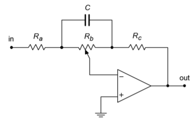
A simple bass control is shown in Figure 2 . To understand how this circuit works, let’s look at what happens at very low and at very high frequencies. First of all, at very high frequencies, capacitor 𝐶 is ideally shorted. Thus, the setting of potentiometer 𝑅𝑏 is inconsequential. In this case, the gain magnitude of the amplifier will be set at 𝑅𝑐/𝑅𝑎 . Normally, 𝑅𝑐 is equal to 𝑅𝑎 , so the gain is unity. At very low frequencies the exact opposite happens; the capacitor is seen as an open. Under this condition the gain of the amplifier depends on the setting of potentiometer 𝑅𝑏 . If the wiper is set to the extreme right, the gain becomes 𝑅𝑐/(𝑅𝑎+𝑅𝑏) . If the wiper is moved to the extreme left, the gain becomes (𝑅𝑐+𝑅𝑏)/𝑅𝑎 . If 𝑅𝑏 is set to nine times 𝑅𝑎 , the total gain range will vary from 0.1 to 10 (−20 dB to +20 dB). A similar arrangement may be used to adjust the treble range.
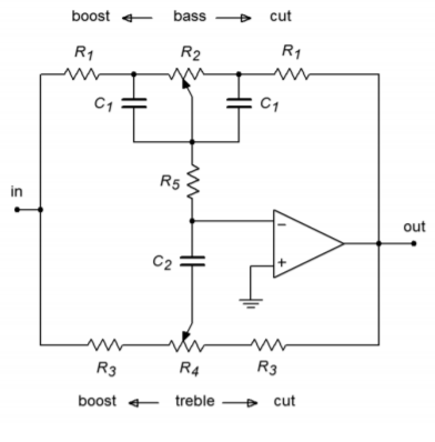
When the bass and treble controls are combined, component loading makes the circuit somewhat more difficult to design. Basic models have already been derived by a number of sources, though, including the one shown in Figure 3 .
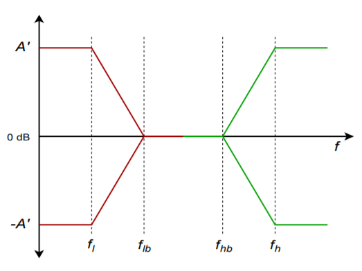
The following equations are used to design the desired equalizer. (Refer to Figure 4 .)
Bass section (assumes 𝑅2≫𝑅1 ):
![\[f_l = \frac{1}{2\pi R_2C_1} \]](https://pressbooks.nscc.ca/app/uploads/quicklatex/quicklatex.com-e13558e9b51a765b74a1176d7b1f32d5_l3.png "Rendered by QuickLaTeX.com")
![\[f_{lb} = \frac{1}{2\pi R_1C_1} \]](https://pressbooks.nscc.ca/app/uploads/quicklatex/quicklatex.com-164a624fcd2e32780dcffa4e8ebea4f4_l3.png "Rendered by QuickLaTeX.com")
![\[A_{vb} = 1+ \frac{R_2}{R_1} \]](https://pressbooks.nscc.ca/app/uploads/quicklatex/quicklatex.com-8e45cab3012b8d445e2e0ea1efd568eb_l3.png "Rendered by QuickLaTeX.com")
Treble section (assumes 𝑅4≫𝑅1+𝑅3+2𝑅5 ):
![\[f_h = \frac{1}{2\pi R_3C_3} \]](https://pressbooks.nscc.ca/app/uploads/quicklatex/quicklatex.com-83d15d69ccc4f72f8a101f82e76a3214_l3.png "Rendered by QuickLaTeX.com")
![\[f_{hb} = \frac{1}{2\pi (R_1 + R_3 + 2R_5) C_3} \]](https://pressbooks.nscc.ca/app/uploads/quicklatex/quicklatex.com-6895b1bb4cf6971f7176778148439da8_l3.png "Rendered by QuickLaTeX.com")
![\[A_{vt} = 1+ \frac{R_1 + 2R_5}{R_3} \]](https://pressbooks.nscc.ca/app/uploads/quicklatex/quicklatex.com-cf540bcff8382157b8e6f8494982113a_l3.png "Rendered by QuickLaTeX.com")
In actuality, it is very common to design these sorts of circuits empirically. In other words, the given equations are used as a starting point, and then component values are adjusted in the laboratory until the desired response range is obtained. Circuits like this may be altered further to include a midrange control. Generally, three adjustments is considered to be the maximum for this type of circuit. An example of a bass-midrange-treble equalizer is shown in the schematic for the Pocket Rocket amplifier in Chapter Six.
Computer Simulation A simple bass equalizer is simulated in Figure 5 . The maximum cut and boost is set to a factor of approximately 10, or 20 dB.


In order to plot the response curves, two AC analysis runs are performed: the first with the potentiometer at maximum, and the second at minimum. The two curves are plotted from 10 Hz up to 10 kHz. These curves are essentially mirror images. In both cases the response above 1 kHz is smooth and reasonably flat. The transition to the cut/boost region occurs in the 100 Hz to 1 kHz range, with nearly full action by 40 Hz. If the plot is re-run with the potentiometer in some other position (say, 25 percent of rotation), some smooth, scaled curve within these two extremes will be plotted. If the potentiometer is set at mid-point, the response will be flat across the entire range.
